- RGB
- CMYK
- HSV
- YUV – for backwards compatibility of the TV broadcast
- monochrome
- shades of gray
- color
- pixel =
- alpha channel
- color palette
- conversion table (pixel = pointer into the table)
- types: grayscale (pallete with shades of gray), pseudocolor (color palette), direct color (three color palettes, one for each part of the color – R/G/B)
- usage
- originally for image transmission over phone lines, suitable for WWW
- sharp-edged line art with a limited number of colors → can be used for logos
- small animations
- not used for digital photography
- color palette, max. 256 colors
- supports “transparent” color
- multiple images can be stored in one file
- supports interlacing
- rough image after 25–50 % data
- we can stop the transmission if it's not the image we wanted
- 4-pass interlacing by lines
- LZW-based compression (actually, it uses LZC)
- pointers … binary code with increasing length
- blocks … up to 255 B
- we can increase the number of possible colors by stacking multiple images on top of another (and using transparent pixels)
- motivation: replace GIF with a format based on a non-patented method (LZW was patented by Sperry Corporation / Unisys)
- color space – gray scale, true color, palette
- alpha channel – transparency
- supports only RGB, no other systems (it was designed for transferring images over the network)
- compression has two phases
- preprocessing – predict the value of the pixel, encode the difference between the real and predicted value (prediction based on neighboring pixels)
- prediction types: none, sub (left pixel), up, average (average of sub and up), Paeth (more complicated formula)
- each line may be processed with a different method
- dictionary compression
- deflate (LZ77)
- preprocessing – predict the value of the pixel, encode the difference between the real and predicted value (prediction based on neighboring pixels)
- supports interlacing
- 7-pass interlacing by blocks of pixels

- single image only, no animation