Zkouška

Introduction, Probability

• rational agent
  • agent – perceives environment through sensors, acts upon environment through actuators
  • rational agent maximizes its expected performance measure
  • in AI 1 we used logical approach; we ignored uncertainty
    • including interface between agent and environment
    • we also ignored self-improvement capabilities
• uncertainty in pure logical approach
  • belief states
    • instead of having state, we have a belief state (set of all possibilities that can be true)
  • drawbacks
    • logical agent must consider every logically possible explanation for the observations (no matter how unlikely they are) → large and complex representations
    • we need to consider arbitrary likely events – have a plan for any situation no matter how unlikely it is
    • sometimes there's no plan which would guarantee the desired result (but the agent still has to act somehow)
  • practical problems (in medicine)
    • laziness – it is too much work to list the complete set of antecedents or consequents and too hard to use such rules
    • theoretical ignorance – medical science has no complete theory for the domain
    • practical ignorance – even if we know all the rules, we may not be able run all the necessary tests
  • that's why we'll use another approach – probability theory
• probability
  • sample space = set of possible worlds $\Omega$
    • $\forall\omega\in\Omega: 0\leq P(\omega)\leq 1$
    • $\sum_{\omega\in\Omega} P(\omega)=1$
  • probability of event = sum of probabilities of possible worlds where the event occurs
    • = unconditional/prior probabilities (priors)
  • conditional/posterior probability
    • $P(a\mid b)=\frac{P(a\land b)}{P(b)}$ whenever $P(b)\gt 0$
    • we take some information (evidence) into account
  • in a factored representation, a possible world is represented by a set of variable/value pairs
    • every variable has a domain
    • a possible world is fully identified by values of all random variables
  • probability of all possible worlds can be represented using a table called a full joint probability distribution
  • $\textbf{P}(\mathrm{Cavity})=\braket{0.2,0.8}$
    • Cavity = true → 0.2
    • Cavity = false → 0.8
  • inclusion-exclusion principle
    • $P(a\lor b)=P(a)+P(b)-P(a\land b)$
• practicality of full joint probability distribution
  • we can do inference by summing up certain cells of the full joint distribution table (= marginalization)
  • using normalization constant $\alpha$ may be helpful
  • drawbacks of inference by enumeration
    • worst-case complexity $O(d^n)$ where $d$ is number of values in domains of each variable
    • we need the same space to store the full joint distribution
  • adding another variable – weather
    • does not influence tooth problems (is independent) → we add another table
    • we can represent the resulting joint distribution using two tables
    • conditional independence can be exploited to further reduce the size of representation (instead of one large table, we use several smaller tables)
  • also, we don't need to store the entire table (probabilities add up to one)
• usually, we are interested in the diagnostic direction P(disease | symptoms)
  • but we know P(disease), P(symptoms), and P(symptoms | disease) … causal direction
  • we use Bayes' rule to get the diagnostic direction
  • it may be better not to store the diagnostic direction as the original probabilities (we base the calculation upon) may change
• Bayes’ rule
  • $P(Y\mid X)=\frac{P(X\mid Y)P(Y)}{P(X)}=\alpha P(X\mid Y)P(Y)$
  • or $P(B_j\mid A)=\frac{P(A\mid B_j)P(B_j)}{\sum_i P(A\mid B_i)P(B_i)}=\alpha P(A\mid B_j)P(B_j)$
• naive Bayes model
  • generally, we can exploit conditional independence by ordering the variables properly
  • naive Bayes model – we assume independence
    • $P(\text{Cause}, \text{Effect}_1, \dots, \text{Effect}_n) = P(\text{Cause})\prod_iP(\text{Effect}_i\mid\text{Cause})$

Bayesian Networks

• Bayesian network
  • DAG; specifies conditional dependence among random variables
  • an efficient way to represent full joint probability distribution by exploiting conditional independence
  • nodes correspond to random variables, arcs describe the dependencies
  • CPT (conditional probability table) for each variable
    • to get full joint distribution, we just multiply the tables
  • 
    • autorem obrázku je Roman Barták
    • proměnné jsou binární, proto má tabulka vždy jen jeden sloupec (druhý sloupec by mohl obsahovat pravděpodobnost, že jev nenastane – lze ho dopočítat z prvního sloupce)
• construction
  • we construct the network based on the selected order
  • usually, we want to use the causal direction (so that we know how to construct the CPTs; also the network will be smaller)
  • the arc should be there if there is a dependence between the variables
    • for $X$ independent on $Y$, it should hold that $P(X\mid Y,Z)=P(X\mid \neg Y,Z)=P(X\mid Z)$
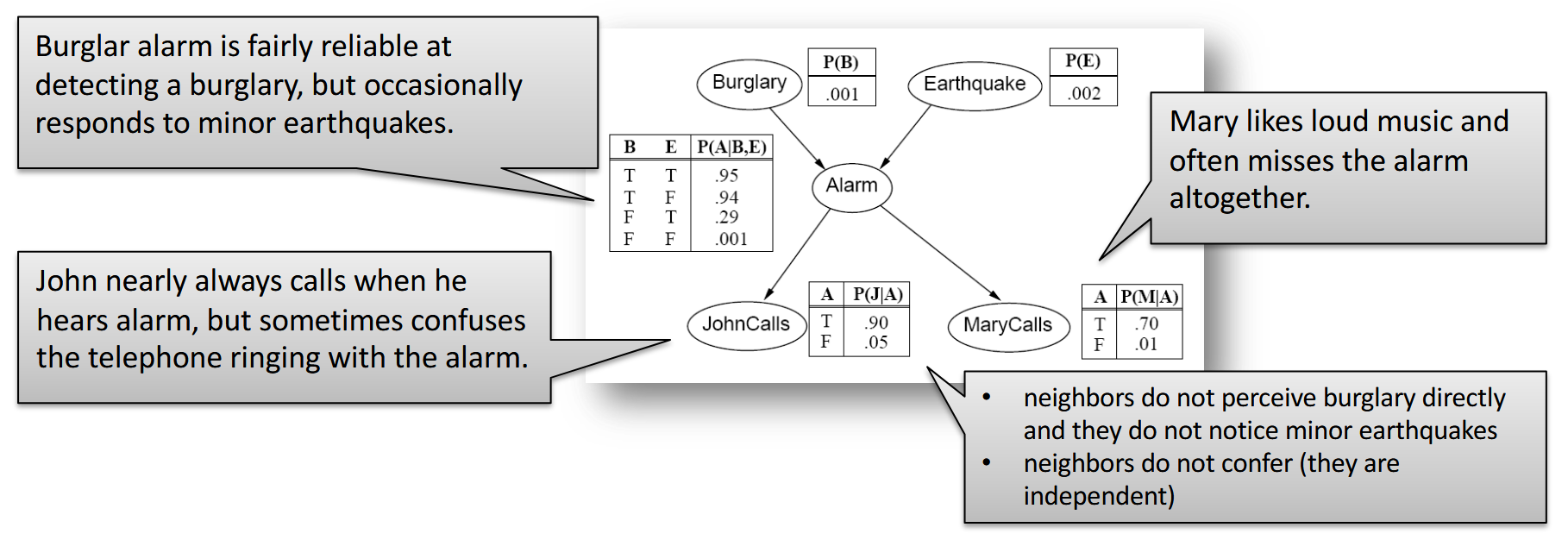
  • příklad: MaryCalls, JohnCalls, Alarm, Burglary, Earthquake (záměrně jdeme od důsledků k příčinám, byť to není praktické)
    • z MaryCalls povede hrana do JohnCalls, protože nejsou nezávislé (když volá Mary, tak je větší šance, že volá i John)
    • z obou povede hrana do Alarmu
    • z Alarmu vedou hrany do Burglary a Earthquake (ale hrany z JohnCalls a MarryCalls tam nepovedou – na těch hranách nezáleží, jsou nezávislé)
    • z Burglary povede hrana do Earthquake, protože pokud zní alarm a k vloupání nedošlo, tak pravděpodobně došlo k zemětřesení
    • akorát se nám v tomto pořadí budou špatně určovat CPT
• how much space can we save?
  • random variables are often influenced by only a few other variables
  • assume that each variable is directly influenced by at most $k$ other variables
  • then the size of representation is $n\cdot 2^k$ for Bayesian network vs. $2^n$ for full joint distribution
  • we can also ignore some slight dependencies – trade-off between accuracy and size of the network
  • we need to choose the correct ordering of variables
• conditional independence in Bayesian networks
  • node is conditionally independent of its non-descendants given its parents
  • node is conditionally independent of all other nodes given its parents, children, and children's parents
    • Markov blanket = parents, children, children's parents
    • M. blanket contains all the information needed to infer the value of the variable (other variables are redundant)
• exact inference (by enumeration)
  • using joint probability (we sum over hidden variables) + moving terms out of the sums if possible
    • $P(X\mid e)=\alpha P(X,e)=\alpha\sum_y P(X,e,y)$
    • kde pravděpodobnost $X$ odvozujeme, $e$ jsou pozorované proměnné (evidence) a $y$ jsou hodnoty další skryté proměnné $Y$
    • přičemž $P(X,e,y)$ lze určit pomocí CPD tabulek
      • když nemůžeme určit konkrétní hodnotu pravděpodobnosti přímo, tak výpočet rozvětvíme
      • některé větve se objeví vícekrát – hodí se nám dynamické programování
    • příklad: $P(b\mid j,m)=\alpha\sum_e\sum_a P(b)P(e)P(a\mid b,e)P(j\mid a)P(m\mid a)$
      • $=\alpha P(b)\sum_e P(e)\sum_a P(a\mid b,e) P(j\mid a)P(m\mid a)$
      • tohle můžeme přímo převést na výpočty s faktory
        • $P(a\mid b,e)$ odpovídá faktoru $f_3(A,B,E)$
        • $P(j\mid a)$ odpovídá faktoru $f_4(A)$, protože hodnotu $j$ známe, tak ji můžeme zafixovat (faktor pak obsahuje tolik čísel, kolik je možných hodnot $A$)
  • we can use factors (tables constructed from CPTs)
    • multiplication: we can (pointwise) multiply the rows that have the same values of the shared variables
    • elimination: we sum the rows that are almost the same (differ only in the value of the variable we want to eliminate)
    • we construct the factors based on the evidence
    • suggested ordering – eliminate the variables that would need large factors in the subsequent stages
  • complexity
    • given by the size of the largest factor constructed
      • heuristic: eliminate whichever variable minimizes the size of the next factor to be constructed
    • if Bayesian network is a polytree (corresponding undirected graph is a tree), then the time and space complexity is linear in the size of the network
      • size of the network = number of CPT entries … $O(nd^k)$
    • 3SAT can be reduced to inference in the Bayesian networks so inference in Bayesian networks is NP-hard
    • the problem is #P-hard (“number of satisfying assignments for a prop. logic formula”)
• approximate inference
  • Monte Carlo methods
  • direct sampling
    • we are going through the Bayesian network in top-down order
    • in each step, we sample one variable and then base further sampling on this choice
    • this only provides us with the samples (but we want to infer the probabilities!)
  • rejection sampling
    • we generate samples using direct sampling
    • we eliminate the ones that don't correspond to the evidence
    • we estimate $P(X\mid e)$ as the number of correct (not eliminated) samples divided by the number of all samples
    • problem: we may reject too many samples
  • likelihood weighting
    • instead of rejecting samples, we generate only the ones consistent with evidence $e$
    • but then, we lose information about the probability of the specific piece of evidence (which may be dependent on the generated hidden variables)
    • so we assign weights to the samples according to the probability of the evidence
    • our arithmetic has to be precise enough
  • MCMC (Markov chain Monte Carlo)
    • start with randomly generated sample consistent with evidence $e$
    • for a selected variable $X$ (outside evidence), select a new value conditioned on the values of the variables in the Markov blanket
    • we get a Markov chain
    • Gibbs sampling
    • sampling process settles into a dynamic equilibrium in which the long-term fraction of time spent in each state is exactly proportional to its posterior probability
    • why it works
      • for stationary distribution we require $\pi(x')=\sum_x \pi(x) q(x\to x')$
      • this holds when $\pi(x) q(x\to x')=\pi(x')q(x'\to x)$ … can be shown
        • $\pi(x)=P(x\mid e)=P(x_i,y_i\mid e)$
        • $q(x\to x')=P(x_i'\mid y_i,e)=P(x_i'\mid mb(X_i))$

Partial Observability

• partially observable environment with discrete time
  • structure of the model is similar to the Bayesian network
  • hidden variables $X_t$, observable variables $E_t$
  • states are evolving according to some rules → transition model
  • Markov assumption: $X_t$ depends on a fixed number of previous states (usually one)
    • $P(X_t\mid X_{0:t-1})=P(X_t\mid X_{t-1})$
    • → first-order Markov chain
      • in a second-order MC, $X_t$ depends on both $X_{t-1}$ and $X_{t-2}$
  • another assumption: the process is stationary
    • transition probabilities are always the same (independent on $t$)
  • sensor Markov assumption: $E_t$ depends only on $X_t$
    • but there are sensors where this does not hold (e.g. liquid-based thermometer)
    • personal note: for proprioceptive sensors, $E_t$ depends on $X_t$ and $X_{t-1}$
  • first-order Markov assumption: the state variables contain all the information needed to characterize the next time slice (its distribution)
    • what if it does not hold?
      • increase the order of the Markov process model or enlarge the set of state variables
      • note: increasing the order can be reformulated as an increase in set of state variables
• inference
  • transition and sensor models can be described using a Bayesian network
    • reasoning in this Bayesian network can be done but is not efficient (too many time steps)
  • basic inference tasks: filtering, prediction, smoothing, most likely explanation
    • these tasks can be performed efficiently without a Bayesian network
    • filtrování (filtering) – znám minulá pozorování, zajímá mě přítomný stav
      • $P(X_{t+1}\mid e_{1:t+1})=P(X_{t+1}\mid e_{1:t},e_{t+1})$
        • použijeme Bayesovo pravidlo
      • $=\alpha\cdot P(e_{t+1}\mid X_{t+1},e_{1:t})\cdot P(X_{t+1}\mid e_{1:t})$
        • použijeme sensor Markov assumption
      • $=\alpha\cdot P(e_{t+1}\mid X_{t+1})\cdot P(X_{t+1}\mid e_{1:t})$
      • $=\alpha\cdot P(e_{t+1}\mid X_{t+1})\cdot \sum_{x_t}P(X_{t+1}\mid x_t,e_{1:t}) P(x_t\mid e_{1:t})$
      • $=\alpha\cdot P(e_{t+1}\mid X_{t+1})\cdot \sum_{x_t}P(X_{t+1}\mid x_t) P(x_t\mid e_{1:t})$
      • užitečný filtrovací algoritmus si musí udržovat odhad současného stavu, jelikož je vzorec rekurzivní
      • používá se forward algoritmus
    • předpověď (prediction) – znám minulá pozorování, zajímají mě budoucí stavy
      • vlastně jako filtering, akorát nepřidávám další pozorování (měření) – používám jenom přechodový model
      • $P(X_{t+k+1}\mid e_{1:t})=\sum_{x_{t+k}} P(X_{t+k+1}\mid x_{t+k}) P(x_{t+k}\mid e_{1:t})$
      • po určitém čase (mixing time) distribuce předpovědí konverguje ke stacionárnímu rozdělení daného markovského procesu a zůstane konstantní
    • vyhlazování (smoothing) – znám minulá pozorování, zajímají mě minulé stavy
      • $P(X_k\mid e_{1:t})=P(X_k\mid e_{1:k},e_{k+1:t})$
        • použijeme Bayesovo pravidlo
      • $=\alpha\cdot P(X_k\mid e_{1:k})\cdot P(e_{k+1:t}\mid X_k,e_{1:k})$
        • použijeme sensor Markov assumption
      • $=\alpha\cdot P(X_k\mid e_{1:k})\cdot P(e_{k+1:t}\mid X_k)$
      • přitom levý člen známe z filteringu (je to „dopředný směr“), pravý je „zpětný směr“ z naměřených hodnot v budoucnosti (relativně vůči danému okamžiku)
        • dostaneme $P(e_{k+1:t}\mid X_k)=\sum_{x_{k+1}} P(e_{k+1}\mid x_{k+1})P(e_{k+2:t}\mid x_{k+1})P(x_{k+1}\mid X_k)$
      • používá se forward-backward algoritmus
    • nejpravděpodobnější vysvětlení (most likely explanation) – znám minulá pozorování, zajímá mě nejpravděpodobnější posloupnost minulých stavů
      • hledáme posloupnost $X_{1:t}$ takovou, že má největší $P(X_{1:t+1}\mid e_{1:t+1})$
      • opět existuje rekurzivní vzorec – podíváme se na pravděpodobnosti předchozích stavů a na nejpravděpodobnější „cesty“ do těchto stavů
      • používá se Viterbiho algoritmus
      • we could do smoothing for every time slice and select the most probable state at the given time
        • but this might lead to a sequence with very low probability (e.g. if there are two states with low transition probability)
      • we don't need to normalize if we only want the maximum (but the numbers get smaller)
      • most likely path to a given state … most likely path to some previous state followed by a transition to the given state
        • $\max_{x_1,\dots,x_t} P(x_1,\dots,x_t,X_{t+1}\mid e_{1:t+1})=$ $\alpha P(e_{t+1}\mid X_{t+1})\max_{x_t} (P(X_{t+1}\mid x_t)\max_{x_1,\dots,x_{t-1}} P(x_1,\dots,x_t\mid e_{1:t}))$
        • forward message passing
• hidden Markov models
  • single discrete random variable & single evidence variable → it's a hidden Markov model
  • we can use matrix implementation of all the basic algorithms
  • transition model … $S\times S$ matrix $T$ s.t. $T_{ij}=P(X_t=j\mid X_{t-1}=i)$
  • sensor model … diagonal matrix $O_t$ s.t. $O_{t\, ii}=P(E_t=e_t\mid X_t=i)$
    • we know the value of the evidence variable $e_t$
  • full smoothing
    • we don't need to run smoothing $t$ times in order to smooth the whole sequence
    • we can use dynamic programming (store the forward/backward values) – but we need more memory then
      • we need to store the whole sequence of forward distributions
    • idea: remember only the current forward distribution, apply operation to get the previous one
      • we can exploit matrix multiplication – use the inverse matrices $(T^T)^{-1},O^{-1}$ if possible (for the $O$ matrix it's always possible as it's a diagonal matrix)
  • smoothing with a fixed time lag
    • $P(X_{t-d}\mid e_{1:t})$
    • forward: simple
    • backward: keep the result in the matrix form
      • then the product of matrices can be modified incrementally (again using inverse matrices)
      • convert it to vector just when using it

Dynamic Bayesian Networks, Kalman Filter

• skryté Markovské modely (HMM) vs. dynamické Bayesovské sítě
  • skryté Markovovy modely
    • předpokládejme, že stav procesu je popsán jedinou diskrétní náhodnou proměnnou $X_t$ (a máme jednu proměnnou $E_t$ odpovídající pozorování)
    • pak můžeme všechny základní algoritmy (filtering, prediction, smoothing, …) implementovat maticově
  • dynamická bayesovská síť
    • umožňuje popsat víc náhodných proměnných
    • reprezentuje časový pravděpodobnostní model
    • zachycuje vztah mezi minulým a současným časovým okamžikem (minulou a současnou vrstvou)
    • každá stavová proměnná má rodiče ve stejné vrstvě nebo v předchozí (podle Markovova předpokladu)
      • stačí nám zachytit jeden slice – prior $P(X_0)$, přechodový model $P(X_1\mid X_0)$, senzorový model $P(E_1\mid X_1)$
  • dynamická bayesovská síť (DBN) vs. skrytý Markovův model (HMM)
    • skrytý Markovův model je speciální případ dynamické bayesovské sítě
    • dynamická bayesovská síť může být kódovaná jako skrytý Markovův model
      • jedna náhodná proměnná ve skrytém Markovově modelu je n-tice hodnot stavových proměnných v dynamické bayesovské síti
      • v HMM vlastně celý stav světa komprimujeme do jedné náhodné proměnné – v DBN jich můžeme mít víc
    • vztah mezi DBN a HMM je podobný jako vztah mezi běžnými bayesovskými sítěmi a tabulkou s full joint probability distribution
      • DBN je výrazně úspornější
      • např. přechodový model u DBN s 20 binárními stavovými proměnnými, kde každá má tři rodiče, obsahuje $20\cdot 2^3=160$ pravděpodobností
      • přechodový model u takového HMM by obsahoval $2^{20}\cdot 2^{20}\approx 10^{12}$ pravděpodobností
• přesná inference v DBNs
  • mohli bychom „rozrolovat“ DBN do plné bayesovské sítě
  • můžeme použít inkrementální přístup – pamatovat si pouze dva slicy (proměnné z minulých sliců můžeme vysčítat)
  • potíž je v tom, že prostor potřebný k uložení největšího faktoru bude exponenciální vzhledem k počtu stavových proměnných … $O(d^{n+k})$
    • $n$ … počet proměnných
    • $k$ … maximální počet rodičů libovolné stavové proměnné
    • $d$ … velikost domény
• přibližná inference v DBNs
  • samplujeme skryté proměnné v síti v topologickém pořadí pomocí likelihood weighting
    • najednou samplujeme $N$ vzorků, procházíme sítí
  • vzorky se generují nezávisle na měření, takže můžou mít hodně nízké váhy a ty s časem klesají
  • abychom udrželi přesnost, musíme počet vzorků exponenciálně zvětšovat v závislosti na $t$
  • chceme se při samplování zaměřit na oblasti sample space s velkou pravděpodobností → použijeme particle filtering
• particle filtering
  • populace $N$ vzorků se vyrobí samplováním z prioru $P(X_0)$
  • každý vzorek se propaguje dopředu tak, že samplujeme pomocí přechodového modelu
  • každý vzorek se váží (likelihood weighting)
  • nakonec resamplujeme populaci vzorků – vyrobíme nevážené vzorky, přičemž každý vzorek vybereme z původní populace tak, že pravděpodobnost jeho výběru je úměrná jeho váze
• sensor failures
  • fully accurate → sensor model is an “identity matrix”
  • Gaussian error model – models measurement noise
  • transient failures × persistent failures
  • sensor transient failure model – we use some inertia that helps to overcome temporary blips in the readings
  • sensor persistent failure model – we use additional state variable that describes the status of the sensor (is it broken?)
• continuous variables
  • so far we assumed discrete random variables (probability distributions can be captured by tables)
  • how to handle continuous variables
    • discretization → loss of accuracy, large CPTs
    • standard families of probability density functions – e.g. normal (Gaussian) distribution
      • $f(x)=\frac 1{\sigma\sqrt{2\pi}}e^{-\frac12(\frac{x-\mu}{\sigma})^2}$
• conditional probability tables for continuous variables
  • dependence of continuous on continuous
    • can be described using a linear Gaussian distribution – mean value as a linear function of the parent, standard deviation is fixed
  • dependence of continuous on discrete
    • specify parameters of standard distribution for each value of the discrete variable
  • dependence of discrete on continuous
    • “soft” threshold function
    • examples
      • probit (probability unit) distribution
        • $\Phi(x)$
        • often a better fit to real situations (the underlying decision process has a hard threshold, but the precise location of the threshold is subject to random Gaussian noise)
      • logit (logistic function) distribution
        • log-odds, inverse of sigmoid
        • has longer tails, may be easier to deal with mathematically
• Kalman filters
  • we use dynamic Bayesian network to model a problem (e.g. localization), we use linear Gaussian distributions both in the transition model and in the sensor model
  • then, everything is Gaussian
  • we can use message passing technique for filtering, prediction, and smoothing
  • what if the model is non-linear?
    • example: bird is heading straight for a tree trunk (linear model predicts a collision)
    • standard solution: switching Kalman filter
    • we run multiple Kalman filters in parallel, each uses a different model of the system
    • we use a weighted sum of predictions – depending on how they fit the current data
    • this is a special case of DBN obtained by adding another discrete state variable to the network (“which filter to use”)
• keeping track of many objects
  • which object generated which observation?
  • exact reasoning → consider all possible assignments ($n!$ mappings for a single time slice)
  • approximate methods
    • choose a single best assignment at each time step
      • naive: nearest-neighbor filter (which observation is the closest to this prediction)
      • better: maximize the joint probability of the current observations gtiven the predicted positions (the Hungarian algorithm)
      • but these methods fail under more difficult conditions (they commit to a single best assignment which may subsequently become clear to be wrong)
    • particle filtering – maintains a large collection of possible current assignments
    • MCMC – explores the space of possible current assignments
  • problems with real applications
    • false alarm (an observation is not caused by a real object)
    • detection failure (no observation reported for a real object)
    • new and disappearing objects (set of objects is not fixed)

Utility Theory

• užitek (utility)
  • pro každý stav známe utility function (funkci užitku) … $U(s)$
  • očekávaný užitek (expected utility, EU) akce $a$, máme-li pozorování $e$
    • $EU(a\mid e)=\sum_s P(\text{Result}(a)=s\mid a,e)\cdot U(s)$
  • maximální očekávaný užitek (maximum expected utility, MEU)
    • $\text{argmax}_a EU(a\mid e)$
  • princip maximálního očekávaného užitku: racionální agent by si měl zvolit akci, která maximalizuje očekávaný užitek agenta
• teorie užitku
  • očekávaný užitek náhodné volby (loterie) … $\sum_i p_i u_i$
    • $p_i$ … pravděpodobnost $i$-té volby
    • $u_i$ … užitek $i$-té volby
  • často známe preference agenta spíše než přesné hodnoty utility funkce
    • $A \lt B$ … agent preferuje B oproti A
    • $A \sim B$ … agent nerozlišuje mezi A a B (nemá favorita, je indiferentní)
  • rational preferences should obey certain constraints
    • orderability
      • agent buď preferuje jednu z voleb, nebo je indiferentní
    • transitivity (violating it can lead to irrational behavior)
    • continuity
      • pokud $A\lt B\lt C$, pak můžeme $A,C$ namíchat v takovém poměru, aby platilo, že je agent indiferentní mezi $B$ a touto novou loterií
    • substitutability
      • pokud $A\sim B$, tak můžeme v loterii nahradit výsledek $A$ výsledkem $B$ a agent bude indiferentní mezi původní a novou loterií
    • monotonicity
      • idea: mějme dvě loterie se stejnou množinou výsledků, pak agent preferuje tu, kde má jeho preferovaný výsledek větší pravděpodobnost
    • decomposability
      • loterie, kde jeden z výsledků je loterií, se dá zploštit do jedné větší loterie
  • z prefencí se dá dostat utility
    • $U(A)\lt U(B)\iff A\lt B$
    • $U(A)=U(B)\iff A\sim B$
    • utility funkce zjevně nemusí být jedinečná
  • alternativní způsob – získáme normalizovanou utility funkci
    • nejlepšímu možnému stavu $S_\text{max}$ přiřadíme $U(S_\text{max}) = 1$
    • nejhorší možné katastrofě $S_\text{min}$ přiřadíme $U(S_\text{min}) = 0$
    • pro každý další stav $S$ necháme agenta rozhodnout se mezi standardní loterií a stavem $S$
      • standardní loterie … $S_\text{max}$ s pravděpodobností $p$ a $S_\text{min}$ s pravděpodobností $1-p$
      • upravujeme pravděpodnost $p$, dokud agent není indiferentní mezi $S$ a standardní loterií
        • pak $U(S):=p$
• utility of money, human judgement
  • problem: take one million now or gamble and potentially get 2.5× more (or zero)?
    • is the expected utility greater in the second case?
  • utility is not a linear function of the money that an agent has
    • if you have billions, one million does not matter that much
  • Allais paradox
    • certainty effect – people are attracted to gains that are certain
    • 80% chance of 4000 USD vs. 100% chance of 3000 USD
    • 20% chance of 4000 USD vs. 25% chance of 3000 USD
  • Ellsberg paradox
    • ambiguity aversion – people prefer the known probability
    • example with balls in an urn
  • framing effect
    • 90% survival rate × 10% death rate (which procedure do you prefer? :D)
  • anchoring effect
    • an expensive product makes cheaper (but still quite expensive) products seem like a good deal
• multi-attribute utility theory: dominance
  • sometimes we can use dominance to select the best outcome without combining the attribute values
    • strict dominance
    • can be used even for uncertained outcomes (instead of individual points, we consider some areas)
    • stochastic dominance
      • best seen by examining the cumulative distribution (does it hold that $\forall t:F_1(t)\leq F_2(t)$?) – for a single variable
• multi-attribute utility theory: preference structure
  • if there are $n$ attributes, each with $d$ values, we may need to have utility values for $d^n$ states
    • but often, there is some level of regularity
  • preference independence
    • two attributes $X_1,X_2$ are independent of a third attribute $X_3$ if the preference between outcomes $\braket{x_1,x_2,x_3}$ and $\braket{x_1',x_2',x_3}$ does not depend on the particular value $x_3$
  • mutual preferential independence (MPI)
    • if each pair of attributes is preferentially independent of any other attribute
    • then $U(x_1,\dots,x_n)=\sum_i U_i(x_i)$
      • additive value function
  • for uncertainty, we need utility independence
    • a set of attributes $X$ is utility independent of a set of attributes $Y$ if preferences between lotteries on the attributes in $X$ are independent of the particular values of the attributes in $Y$
  • mutually utility independent (MUI) attributes
    • multiplicative utility function $U=k_1U_1+k_2U_2+k_3U_3+k_1k_2U_1U_2+k_2k_3U_2U_3+k_1k_3U_1U_3+k_1k_2k_3U_1U_2U_3$
• the value of information
  • “what questions to ask?”
  • value of perfect information (VPI)
    • we consider expected utility before and after getting the information (expected value over any possible information we could get)
  • expected value of information
    • non-negative
    • not additive
    • order independent
  • information gathering – how should rational agent proceed
    • ask questions in reasonable order
    • avoid asking irrelevant questions
    • consider cost of each piece of information and its importance
    • stop asking when it's appropriate
  • qualitative value of information
    • information is beneficial if it changes my action
    • how much do I gain by changing my action?

Sequential Decision Problems

• decision network
  • what it contains
    • chance nodes – random variables
    • decision nodes – points where the decision maker has a choice of actions
    • utility nodes – agent's utility function
  • evaluating it
    • we set the evidence variables for the current state
    • for each possible value of the decision node…
      • we set the decision node to that value
      • we calculate the posterior probabilities of the chance nodes
      • we calculate the resulting utility
    • we return the action (decision) with the highest utility
  • multiple utility nodes → multi-attribute utility theory
  • in practice
    1. create a causal model
    2. simplify to a qualitative decision model
    3. assign probabilities
    4. assign utilities
    5. verify and refine the model
    6. perform sensitivity analysis
• sequential decision problems
  • we consider a fully observable environment with unreliable actions (stochastic environment)
  • Markov decision process
    • transition model $P(s'\mid s,a)$
      • Markovian (probability does not depend on the history)
    • utility function depends on a sequence of states
    • is additive
  • how to set the utility (example)
    • goal exit: +1
    • unwanted exit: -1
    • other states: -0.04 (to find the shortest path to the goal)
• solution to a MDP = policy
  • finite sequence of actions cannot be used in stochastic environment, we need a policy function $\pi(s)$
  • optimal policy – yields the highest expected utility
  • a policy describes a simple reflex agent
  • time horizon – two possibilities (we assume the second one)
    • finite time horizon
      • utilities of states could change over time
      • optimal policy could be nonstationary
    • infinite horizon
      • there is no reason for the same state to have different utility at two different moments
      • optimal policy is stationary
  • we assume that the utility (agent's preference) does not change
  • how to assign utilities to sequences
    • additive rewards: $U(s_0,s_1,s_2,\dots)=R(s_0)+R(s_1)+R(s_2)+\dots$
    • discounted rewards: $U(s_0,s_1,s_2,\dots)=R(s_0)+\gamma R(s_1)+\gamma^2 R(s_2)+\dots$
      • discount factor $\gamma\in(0,1)$
      • rewards in the distant future are viewed as insignificant
      • we will use this
        • we can work with environments without a terminal state
  • policy that always reaches a terminal state = proper policy (we can use additive rewards then)
  • infinite sequences can be compared in terms of average reward obtained per time step
  • for our infinite situation
    • policy is driven by the current state and the goal
    • it does not depend on the initial state of the agent
  • instead of reward in a given state $R(s)$, it is useful to define the true utility of a state as $U(s)=U^{\pi^*}(s)$ … expected utility of the optimal policy if the agent starts from the state $s$
• Bellmanova rovnice
  • opravdový užitek stavu je reward (odměna) stavu ve spojení se střední hodnotou užitku následného stavu → to vede na Bellmanovu rovnici
  • vezmu reward a discountovaný užitek okolí
  • akorát nevím, kterou akci provedu, tak vezmu všechny a maximum přes ně (násobím jejich užitek pravděpodobností)
  • $U(s)=R(s)+\gamma\max_a\sum_{s'}P(s'\mid s,a)\ U(s')$
• iterace hodnot, iterace strategií
  • předpoklad: známe reward $R$ a transition model $P$
    • chceme najít užitek $U$ nebo optimální strategii $\pi$
  • soustava Bellmanových rovnic není lineární – obsahuje maximum
    • můžeme je řešit aproximací
    • použijeme iterativní přístup
      • nastavíme nějak užitky – třeba jako nuly
      • provedeme update – aplikujeme Bellmanovu rovnici
      • iterujeme, dokud to nezkonverguje
    • → value iteration
    • proč to funguje?
      • ta funkce („aplikace Bellmanovy rovnice“) má jeden pevný bod
      • s každou iterací se chyba zmenší aspoň o $\gamma$
  • strategie se ustálí dřív než užitky (užitky nemusíme znát přesně, abychom dovedli říct, který stav je lepší)
    • policy loss … vzdálenost mezi užitkem optimální a současné strategie
    • můžeme iterativně zlepšovat policy, dokud to jde
    • → policy iteration
    • z rovnic nám zmizí maximum (protože akci nám fixuje policy) → máme lineární rovnice
      • policy evaluation = nalezení řešení těchto rovnic (tak najdeme utilities stavů)
      • gaussovka je $O(n^3)$
      • u velkých stavových prostorů dává smysl k policy evaluation použít value iteration
    • algoritmus doběhne, protože policies je jenom konečně mnoho (pro konečný stavový prostor) a vždycky hledáme tu lepší
• POMDP
  • máme přechodový model $P(s'\mid s,a)$, akce $A(s)$ i odměny $R(s)$
  • navíc nám přibude sensor model $P(s\mid e)$
  • místo reálných stavů můžeme používat ty domnělé (belief states)
    • pravděpodobnostní distribuce
  • nový belief state $b'$ po použití akce $a$ se spočítá pomocí filteringu
  • policy je funkce, která pro daný belief state $b$ vrátí akci
  • reward … $r(b)=\sum_s b(s) R(s)$
  • POMDP can be reduced to a continuous-space MDP (which is usually multi-dimensional)
    • $P(b'\mid b,a)$ and $r(b)$ define an observable MDP
    • there are infinitely many states (each MDP state corresponds to one possible belief state of the POMDP)
  • value iteration can be modified for POMDPs but it's not very efficient
  • dynamic Bayesian networks and look-ahead techniques are more efficient
    • modely přechodů a senzorů jsou reprezentovány dynamickou bayesovskou sítí
    • přidáme rozhodování a užitky, čímž dostaneme dynamickou rozhodovací síť
    • expected minimax algorithm
      • generujeme si stromeček, kde se střídají vrstvy akcí a belief states
      • depth of search tree can be determined by the discount factor

Game Theory, Mechanism Design

• základy teorie her
  • jednou z úloh teorie her je volba vhodné strategie – tedy návodu, jak hru hrát
    • uvažujeme hry v normálním tvaru: hru tvoří hráči, jejich akce a užitkové funkce
    • hráči táhnou zároveň, každý provede jedinou akci
    • strategie může být čistá (přímo konkrétní akce) nebo smíšená (pravděpodobnostní rozdělení přes akce)
  • díváme se na optimalitu strategie nebo strategického profilu (množiny strategií všech hráčů) z různých úhlů pohledu
    • strategie $s_1$ dominuje strategii $s_2$, pokud při volbě $s_1$ získá hráč větší užitek než při volbě $s_2$ nehledě na strategie ostatních hráčů
      • strategie je dominantní, pokud dominuje všechny ostatní strategie
      • když má každý hráč dominantní strategii, jejich kombinace se nazývá dominant strategy equilibrium
    • Nashovo ekvilibrium je takový strategický profil, že by žádný hráč neměnil svou strategii, kdyby znal strategie ostatních
      • existuje v každé hře
    • strategický profil $s$ Pareto dominuje profil $s'$, pokud si změnou z $s'$ na $s$ žádný hráč nepohorší, ale aspoň jeden hráč si polepší
      • strategický profil je Pareto optimální, pokud neexistuje profil, který by ho Pareto dominoval
    • další zajímavým typem ekvilibria je korelované ekvilibrium
  • vězňovo dilema
    • dva hráči (vězni)
    • vězeň může vypovídat (testify/defect) nebo odmítnout vypovídat (refuse/cooperate)
      • oba vypovídají → oba ztrácejí málo (užitek -5)
      • jeden vypovídá, druhý ne → jeden neztratí nic (užitek 0), druhý hodně ztratí (užitek -10)
      • oba odmítnou → oba ztrácejí velmi málo (užitek -1)
    • vypovídat je čistá dominantní strategie
      • ale když vypovídají oba hráči, tak vyhrála policie – lepší by bylo, kdyby oba odmítli vypovídat
      • našli jsme Nashovo ekvilibrium – nikdo neprofituje ze změny strategie, pokud druhý hráč zůstane u stejné strategie
• maximin
  • dvouprstá Morra nemá čistou strategii
  • jak najít optimální smíšenou strategii?
    • technika maximin (vyvinul ji von Neumann)
    • nejdříve si představíme, jak by se hra hrála, kdyby se hráči střídali a kdyby hráli čistou strategii (obě varianty – podle toho, který hráč začíná)
    • minimaxem vyhodnotíme strom hry
    • získáme spodní a horní mez pro skóre
    • teď si představíme, že hráči mají smíšenou strategii s nějakou pravděpodobností $p$, a uděláme to samé
    • spočítáme lineární rovnice
    • tak najdeme Nashovo ekvilibrium
      • v případě Morry bychom s pravděpodobností 7/12 měli ukázat jeden prst a s pravděpodobností 5/12 dva prsty
      • lichý hráč je na tom lépe
• opakované hry
  • známe historii tahů, payoff se sčítá
  • strategie pro opakované vězňovo dilema
    • pokud víme, která hra je poslední, vede to na podobnou situaci jako u jedné hry
    • pokud nevíme, která hra je poslední
      • perpetual punishment – hráč odmítá vypovídat, právě když druhý hráč nikdy nevypovídal
      • tit-for-tat – hráč nejprve odmítá vypovídat, pak zrcadlí pohyby protivníka
        • velmi robustní a efektivní strategie
• mechanism design (inverse game theory)
  • mechanism consist of…
    • language for describing the set of strategies that agents may adopt
    • center (a distinguished agent) – collects reports of strategy choices from the remaining agents
    • outcome rule – used to determine the payoffs given strategy choices
  • aukce obecně
    • každý agent $i$ přiřazuje věci hodnotu $v_i$, nabízí za ni $b_i$ (bid)
    • $b_i\leq v_i$
  • jak se pozná dobrý mechanismus aukce
    • maximalizuje výnos pro prodejce
    • vítěz aukce je agent, který si věci nejvíc cení (mechanismus je efektivní)
    • zájemci by měli mít dominantní strategii – obvykle je to truth-revealing strategie (zájemce nabízí $b_i=v_i$)
• typy aukcí
  • anglická aukce (ascending-bid)
    • začnu s $b_\text{min}$, pokud je to nějaký zájemce ochotný zaplatit, tak se ptám na $b_\text{min}+d$
    • strategie: přihazuju, dokud cena není vyšší než moje hodnota
      • jednoduchá dominantní strategie
    • má to problémy
      • není truth-revealing: u vítěze známe jenom dolní odhad jeho $v_i$
      • nepůjdu do aukce s někým hodně bohatým
        • to je problém i pro prodejce, protože to může vést k situaci, kdy se věc prodá za $b_\text{min}$
      • lidi musejí být ve stejnou chvíli na stejném místě (nebo komunikovat rychle a bezpečně)
      • collusion = an unfair or illegal agreement by two ore more bidders to manipulate prices
        • example: Mannesman and T-Mobile (they both got half of the available blocks)
  • holandská aukce
    • začíná se vyšší cenou, snižuje se, dokud ji někdo nepřijme
    • je rychlá
  • obálková aukce
    • největší nabídka vítězí
    • neexistuje jednoduchá dominantní strategie
      • pokud věříš, že maximum ostatních nabídek je $b_0$, tak bys měl nabídnout $b_0+\varepsilon$, pokud je to menší částka než tvoje $v_i$
    • agent s nejvyšší $v_i$ již nemusí vyhrát aukci
      • aukce je „kompetitivnější“
  • obálková second-price aukce (Vickrey)
    • vyhraje ten první, platí druhou cenu
    • dominantní strategie je tam dát svoji hodnotu $v_i$
      • lze to ukázat rozborem případů, zda je $v_i-b_0$ větší nebo menší než nula (vždycky je optimální nabídnout $v_i$)
      • $b_0$ … druhá nejlepší nabídka
• problém sdílení společných zdrojů
  • znečišťování životního prostředí
    • pokračovat ve znečišťování je levnější než implementovat potřebné změny
  • „tragedy of commons“ (tragédie občiny)
    • když nikdo nemusí platit za sdílený zdroj, může to vést k jeho využívání tím způsobem, že se snižuje utilita pro všechny agenty
    • podobné vězňovu dilematu
• mechanismus Vickrey-Clarke-Groves (VCG)
  • příklad: rozdělení (a zdanění) společného zboží
  • princip
    • každý agent nahlásí svoji hodnotu (nabídku)
    • centrální autorita přiřadí zboží podmnožině agentů tak, aby se maximalizoval celkový nahlášený užitek
    • každý vítězný agent platí daň odpovídající nejvyšší nahlášené hodnotě mezi těmi, kdo prohráli
  • dominantní strategie je opravdu nabídnout svoji hodnotu
  • VCG lze použít i ve velmi obecných případech
    • obecně: výše platby odpovídá tomu, jakou ztrátu sociálního zisku způsobuje $i$-tý zájemce ostatním (tzn. o kolik poklesne součet $v_i$ pro ostatní vítězné agenty, když se $i$-tý agent přidá do aukce)
  • problém: je nezbytné mít centrální autoritu
  • vede to k optimálnímu výsledku?
    • vítězové jsou šťastní, protože platí méně než $v_i$
    • poražení jsou šťastní, protože jejich $v_i$ je nižší, než by museli platit
  • je to truth-revealing?
    • chci maximalizovat $v_i+\sum_{j\neq i}b_j-W_{-i}$
    • ale $W_{-i}$ (tj. celkovou utilitu bez hráče $i$) nemůžu ovlivnit
    • pak chci maximalizovat $v_i+\sum_{j\neq i}b_j$, což přesně maximalizuje alokační pravidlo, pokud $b_i=v_i$

Supervised Learning

• strojové učení
  • způsob, jak zlepšit budoucí chování agenta
  • co učení zvládá lépe než přímé programování chování
    • scénáře, na které programátor nemyslel
    • změny v prostředí
    • někdy není jasné, jak agenta naprogramovat
  • zpětná vazba, z nichž se agenti učí
    • učení bez učitele (unsupervised learning) – agent se učí vzory ve vstupu, aniž by měl nějakou explicitní zpětnou vazbu
    • zpětnovazební učení (reinforcement learning) – agent dostává odměny nebo tresty
    • učení s učitelem (supervised learning) – agent se učí funkci, která mapuje vstupy na výstupy
• učení s učitelem (supervised learning)
  • máme vstupy a výstupy
  • chceme najít funkci (její aproximaci), která mapuje vstupy na výstupy
  • hledáme hypotézu (funkci $h$) z prostoru hypotéz
  • hypotéza je konzistentní s $i$-tým příkladem, pokud $h(x_i)=y_i$
  • princip Occamovy břitvy – preferujeme nejjednodušší hypotézu
    • např. $n$ bodů určuje polynom stupně $n-1$, ale pokud body leží na přímce, tak nejjednodušší hypotéze je prostě ta přímka
  • typy úloh
    • klasifikace – u nečíselných funkcí, data rozdělujeme do množin
    • regrese – u číselných funkcí
• decision trees
  • for binary variables … $2^n$ possible input vectors, each can be mapped to 0 or 1
    • so we get $2^{2^n}$ hypotheses
  • constructed using a greedy divide-and-conquer strategy
  • if we have no remaining attributes and there are still multiple classes, we return the mode (majority vote, česky modus)
  • if there are no samples in the branch of the tree, we use the default value (class) = mode at the previous level
  • to find the best splitting attribute, we use information gain (decrease of Shannon entropy)
    • we subtract the weighted average of new entropies (in the branches) from the original entropy
  • chance of overfitting increases with the number of hypotheses
  • decision tree pruning
    • bottom-up approach, $\chi^2$ test
      • take a test node that has only leaf nodes as descendants
      • null hypothesis: there is no underlying pattern (the node is testing an irrelevant attribute)
    • can it be used when constructing the decision tree as an early-stopping condition?
      • no, there are cases where we need a combination of attributes to classify (e.g. XOR) but individual attributes would fail $\chi^2$
  • problems
    • missing data
      • usually, we use the most frequent value (mode) to fill the missing one
    • multivalued attributes
      • traditionally, we consider nominal attributes with several possible values – what if we have integers or real numbers?
      • find a threshold
      • for real values, we may want to sort the samples and look at the points where the class changes
  • can be used for regression
    • but the learning algorithm needs to move from classification to regression at some point (usually, we consider only constants in leaves)
• regression
  • hypothesis space = linear functions
  • univariate linear regression
    • $L_2$ loss
    • we can use an analytical solution – set derivatives equal to zero
    • or we can use gradient descent (works even if the hypotheses are non-linear)
  • multivariate linear regression
    • similar to univariate
    • again, analytical solution or gradient descent
• linear classifiers
  • linear separator – “passing the linear function $wx$ through a threshold function”
  • perceptron learning rule … $w_i\leftarrow w_i+\alpha(y-h_w(x))\cdot x_i$
  • logistic threshold function … $\sigma(z)=\frac 1{1+e^{-z}}$
• non-parametric models
  • “let the data speak for themselves”
  • table lookup
    • the simplest way to learn a function
    • just find the $x$ in the table (if it exists) and return the corresponding $y$
  • $k$-nearest neighbors
    • majority vote ($k$ should be odd)
    • we need to measure distance – usually $L_p$ norm (Minkowski distance)
      • Manhattan distance, Euclidean distance
      • special case: for boolean attribute values, we have Hamming distance (number of attributes where the data points differ)
      • we have to be careful about the scale, it's common to apply normalization for the individual attributes (to zero mean, unit variance)
    • the curse of dimensionality
      • in low-dimensional spaces with plenty of data, nearest neighbors work well
      • as the number of dimension rises, the nearest neighbors may actually be quite far away
      • with more dimensions, we need more data
    • looking for neighbors
      • table lookup… $O(N)$
      • binary tree … $O(\log N)$
        • note that the neighbors might be at different branches
        • works fine if the number of examples is exponential in the number of attributes
      • hash table … $O(1)$
        • we need the hash function to have some special property (locally-sensitive hash)
  • regression: simple approaches
    • we get a piece-wise linear function if we connect all the known points
    • 3-nearest neighbors average
    • 3-nearest neighbors linear regression (we fit a model to the three points closest to our input)
    • locally weighted regression – data points are weighted by their distance
      • resulting curve looks quite smooth actually
  • support vector machines (SVM)
    • three properties
      • maximum margin separator
        • provides good generalization
        • can be found using quadratic programming (via dual representation)
        • is defined by the points closest to the boundary
          • for all the other points, the weights $\alpha_j$ are zero
        • separator … $h(x)=\mathrm{sign}(\sum_j\alpha_j y_j(xx_j)-b)$
      • kernel trick (solves the problem of the data not being linearly separable)
        • we map the data points via $F$ to a higher-dimensional space where they are linearly separable
        • it turns out that we can often compute $F(x_j)F(x_k)$ without computing $F(x_j),F(x_k)$ separately
          • e.g. polynomial kernel $(1+x_jx_k)^d$ … $F$ would be a mapping producing polynomial features of degree $\leq d$
      • it is nonparametric
• ensemble learning
  • we are using multiple hypotheses to perform predictions (they vote)
  • boosting
    • $k$ rounds
    • in every round we generate a hypothesis based on the data, then we increase weights of the misclassified samples (and decrease points of the correctly classified ones)
    • the following hypotheses are generated based on the weighted data
    • even if the underlying algorithm is weak, we can get quite a good classifier
    • AdaBoost algorithm

Logical Formulation of Learning

• logical formulation of learning
  • attributes → unary predicates
  • classification is given by literal using the goal predicate
  • hypothesis: $\forall x:\mathrm{Goal}(x)\iff C_j(x)$
    • $C_j$ … extension of the predicate (this is what we consider to be our hypothesis from now on)
  • hypothesis space … set of all hypothesis
    • hypotheses that are not consistent with the examples can be ruled out
    • two ways to be inconsistent: false negative, false positive
• current-best-hypothesis
  • we start with a simple hypothesis (formula $C(x):=\mathrm{True}$; or we could probably use False)
  • we iterate over the data points and maintain a hypothesis that is consistent with them
    • we may need to generalize the hypothesis (if there is a false negative) or specialize it (if there is a false positive)
    • when generalizing, we prefer removing an item from a conjunction over adding a disjunction – we want to keep the hypothesis as simple as possible (according to Ockham's razor principle)
  • after each modification of the hypothesis, we need to check all the previous examples
    • we may need to backtrack (if no simple modification of the hypothesis is consistent with all the data)
    • problem: strong commitment
      • we have to choose a single hypothesis
• alternative approach: least-commitment search (version space learning)
  • version space learning algorithm / candidate elimination algorithm
  • we process the individual examples and move the boundaries of the version space accordingly
    • $G$ … most general boundary (initially True)
    • $S$ … most specific boundary (initially False)
    • both are sets of hypotheses
  • update (for each example)
    • false negative for $S_i$ → replace $S_i$ in the $S$-set by all its immediate generalizations
    • false positive for $S_i$ → throw $S_i$ out of the $S$-set
    • false positive for $G_i$ → replace $G_i$ in the $G$-set by all its immediate specializations
    • false negative for $G_i$ → throw $G_i$ out of the $G$-set
  • in the end…
    • we have exactly one hypothesis left
    • or the version space collapses (one of the boundaries becomes empty)
    • or we run out of examples and have several hypothesis remaining in the version space
      • → disjunction of hypotheses
      • if they disagree in classification (?), we can perform majority vote
  • note that if there are two samples with the same attributes but different classes, our version space collapses
    • it may happen due to noise or if some important attribute is missing from the data
  • if we allow unlimited disjunctions in the hypothesis space
    • $S$-set will always contain a single most-specific hypothesis (disjunction of positive examples)
    • $G$-set will always contain the negation of the disjunction of the negative samples
    • solution: generalization hierarchy (e.g. $\mathrm{WaitEstimate}(x,30\dots 60)\lor \mathrm{WaitEstimate}(x,\gt 60)$ can be replaced by $\mathrm{LongWait}(x)$)
• inductive logic programming
  • examples are given like Prolog facts
  • classifications are given by Prolog facts
  • we have some background knowledge (in the form of a formula)
  • we want to learn some hypothesis
  • top-down learning
    • we start with an empty clause (as general as possible, needs to be specialized)
    • we add literals to the body one at a time (according to our examples)
      • we need to add them in a way that our clause covers the positive examples and no negative examples
      • we prefer the specialization that classifies correctly more examples
      • the choice of literal can be based on information gain
    • system FOIL – it was able to learn quicksort
  • inverse resolution
    • we are trying to construct the resolution tree backwards
    • it involves a search, each step is non-deterministic (e.g. we may choose more or less general assignments of variables)
    • first step (last in the resolution) – empty resolvent and the negation of the goal (as $C_2$)
      • we need to find $C_1$ which resolves with $C_2$ into $\square$

Learning Probabilistic Models

• Bayesian learning
  • we observe values $d$
  • we have some hypotheses and we know $P(d\mid h_i)$ and $P(h_i)$ for each of them
    • $P(h_i)$ … hypothesis prior
    • $P(d\mid h_i)$ … likelihood of the data
  • then we can make prediction about an unknown quantity $X$
    • $P(X\mid d)=\sum_i P(X\mid d,h_i)\ P(h_i\mid d)=\sum_i P(X\mid h_i)\ P(h_i\mid d)$
    • where $P(h_i\mid d)=\alpha P(d\mid h_i)\ P(h_i)$
  • Bayesian prediction eventually agrees with the hypothesis – posterior probability of any false hypothesis vanishes (for large amounts of observations)
  • Bayesian prediction is optimal (whether the dataset is small or large) – any other prediction is expected to be correct less often
  • for real learning problems, the hypothesis space is usually very large or infinite
    • → we need some approximate or simplified methods
• MAP learning
  • we make prediction based on a single most probable hypothesis (maximum a posteriori)
  • $h_{MAP}=\mathrm{argmax}_{h_i}\ P(h_i\mid d)=\mathrm{argmax}_{h_i}\ P(d\mid h_i)\ P(h_i)$
  • we assume that $P(X\mid d)\approx P(X\mid h_{MAP})$
  • at some point, we solve a maximization problem (instead of large summation or integration problem which is solved in Bayesian learning)
• overfitting
  • Bayesian and MAP learning use the prior to penalize complexity (more complex hypotheses have a lower prior probability)
  • if $H$ contains only deterministic hypotheses ($P(d\mid h_i)$ can only be one or zero), then $h_{MAP}$ is the simplest logical theory that is consistent with the data (= Ockham's razor)
• MDL learning
  • $h_{MAP}=\mathrm{argmax}_{h_i}\ P(d\mid h_i)\ P(h_i)=\mathrm{argmin}_{h_i}(-\log_2 P(d\mid h_i)-\log_2 P(h_i))$
  • $-\log_2 P(h_i)$ … number of bits required to specify the hypothesis $h_i$
  • $-\log_2 P(d\mid h_i)$ … number of bits required to specify the data given the hypothesis
  • MAP learning = choosing the hypothesis that provides maximum compression of data
  • a more direct approach: minimum description length (MDL) learning method
    • we count the bits in binary encoding of the hypotheses and data and select the hypothesis with the smallest number of bits
• maximum-likelihood hypothesis (ML learning)
  • we assume a uniform prior, we only maximize $P(d\mid h_i)$
  • provides a good approximation to Bayesian and MAP learning when the dataset is large (but has a problem with small datasets)
• maximum-likelihood parameter learning
  • we have a Bayesian network with a given structure
  • we want to fill the CPTs correctly
  • we write down an expression for the likelihood of the data as a function of the parameters
    • differentiate the likelihood (or log likelihood usually) with respect to each parameter
    • find the parameter values s.t. the derivatives are zero (this leads to numerical optimization or gradient descent etc.)
  • ML parameter learning problem for a Bayesian network decomposes into separate learning problems – one for each parameter
• naïve Bayes model
  • can be represented as a Bayesian network where class $C$ is the root and attributes $X_i$ are the leaves (direct descendants of the root)
  • for Boolean variables, we have two parameters per leaf + one parameter in the root
    • $P(C=\mathrm{True})$
    • $\forall i:P(X_i=\mathrm{True}\mid C=\mathrm{True})$
    • $\forall i: P(X_i=\mathrm{True}\mid C=\mathrm{False})$
  • $P(C\mid x_1,\dots,x_n)=\alpha P(C)\prod_i P(x_i\mid C)$
  • properties
    • scales well to large models
    • no difficulty with noisy or missing data
    • gives probabilistic predictions
• importance of hidden variables
  • example: medical records include the observed symptoms, the diagnosis, and the treatment applied, they seldom contain a direct observation of the disease itself
  • could we construct a model without the hidden variable (disease, in our example)?
    • yes, but it would dramatically increase the number of parameters
• EM algorithm
  • learning the conditional distribution of the hidden variable without knowing the value of that variable
  • steps
    • pretend that we know the parameters of the model
    • infer the expected values of hidden variables to complete the data
    • update the parameters to maximize likelihood of the model
    • iterate until convergence
  • example
    • candies from two bags, Bag is a hidden variable, we have a naïve Bayes model
    • at the beginning, we somehow initialize the parameters of the model
    • repeat
      • according to the parameters, we compute the expected number of candies in each bag (we also need to compute the expected number of candies with given attributes)
        • e.g. $N(c)=\sum_i P(c\mid \mathrm{attributes}_i)$
        • where $\mathrm{attributes}_i$ … attributes of the $i$-th item in the dataset
      • we update all the parameters according to the computed expected numbers (to maximize likelihood of the model)
        • e.g. $P(c)=N(c)/N$

Reinforcement Learning

• návrhy agentů
  • utility-based agent – naučí se užitkovou funkci, používá ji k volbě akcí
  • Q-learning agent – naučí se Q-funkci („užitek akce“)
  • reflexní agent – naučí se policy, která pro stav vrací akci
• pasivní zpětnovazební učení
  • uvažujeme agenta, který se účastní MDP (markovského rozhodovacího procesu)
  • pasivní učení – známe strategii $\pi$ (je pevně daná) a učíme se, jak je dobrá (učíme se utility funkci)
  • agent nezná přechodový model ani reward function
  • jak najít užitkovou funkci: přímý odhad, ADP, TD
  • přímý odhad utility
    • máme trace (běh) mezi stavy, z toho počítáme utility function
    • odhadujeme užitky jednotlivých stavů
      • užitek stavu = reward-to-go (tedy střední hodnota odměny tohoto a všech budoucích stavů)
      • odměny z budoucích stavů bychom mohli zohledňovat s discount faktorem $\gamma$ (viz výše)
    • užitky pro jednotlivé stavy prostě průměrujeme
      • tzn. na konci každého běhu pro konkrétní výskyt stavu $s$ v tom běhu vezmeme všechny odměny od tohoto výskytu dál a posčítáme je
      • výsledek započteme do running average (pro $s$)
    • v podstatě učení s učitelem – na vstupu je stav, na výstupu užitek stavu (neboli reward-to-go)
    • nevýhoda
      • utilities nejsou nezávislé, ale řídí se Bellmanovými rovnicemi
      • hledáme v prostoru hypotéz, který je výrazně větší, než by musel být (obsahuje spoustu funkcí, co porušují Bellmanovy rovnice) → algoritmus konverguje pomalu
  • adaptivní dynamické programování (ADP)
    • agent se učí přechodový model a odměny $R(s)$
    • přechodový model odhaduje přímo z pozorovaných přechodů
    • utilitu $U$ počítá z Bellmanových rovnic třeba pomocí value iteration
      • využíváme toho, že užitky nejsou nezávislé
    • ADP zajišťuje, že jsou odhady užitků konzistentní
  • temporal-difference (TD) learning
    • upravuje stav, aby odpovídal aktuálně pozorovanému následníkovi
    • když dojde k přechodu ze stavu $s$ do stavu $s'$, tak na $U^\pi(s)$ použijeme update: $U^\pi(s)\leftarrow U^\pi(s)+\alpha\cdot (R(s)+\gamma\cdot U^\pi(s')-U^\pi(s))$
      • $\alpha$ je learning rate
    • vlastnosti
      • nepotřebuju přechodový model (je to model-free metoda)
      • konverguje to pomaleji než ADP
      • provádíme jemné lokální updaty (proto máme learning rate)
• aktivní zpětnovazební učení: obecný princip
  • uvažujeme agenta, který se účastní MDP (markovského rozhodovacího procesu)
  • aktivní učení – agent se učí strategii (policy; jak se rozhodovat) a taky utility funkci
  • mohli bychom použít ADP, tím vznikne hladový agent, který opakuje zažité vzory (nezkouší nové věci)
  • jak může volba optimální akce vést k suboptimálním výsledkům?
    • naučený model není stejný jako reálné prostředí
    • akce nejsou pouze zdrojem odměn, ale také přispívají k učení – ovlivňují vstupy
    • zlepšováním modelu se postupně zvětšují odměny, které agent získává
  • je potřeba najít optimum mezi exploration a exploitation
    • pure exploration – agent nepoužívá naučené znalosti
    • pure exploitation – riskujeme, že bude agent pořád dokola opakovat zažité vzory
    • základní myšlenka: na začátku preferujeme exploration, později lépe rozumíme světu, takže nepotřebujeme tolik prozkoumávat
• aktivní zpětnovazební učení: exploration policies
  • první možná exploration policy: agent si zvolí náhodnou akci s pravděpodobností $\frac1t$ (kde $t$ je čas), jinak se řídí hladovou strategií
    • nakonec to konverguje k optimální strategii, ale může to být extrémně pomalé
  • rozumnější přístup je přiřadit vyšší odhad utility akcím, které agent ještě dostatečně nevyzkoušel
    • použijeme optimistický odhad utility $U^+(s)\leftarrow R(s)+\gamma\max_a f(\sum_{s'}P(s'\mid s,a)\ U^+(s'),N(s,a))$
    • $f(u,n)$ … exploration function (určuje trade-off mezi zvědavostí a hladem)
      • např. by od určitého počtu navštívení mohla vracet $u$ a do té doby by mohla vracet nejlepší možnou odměnu, která by se mohla někde v grafu objevit (aby nás motivovala navštívit všechny stavy)
    • vpravo taky používáme $U^+$ – to nám samo o sobě zajišťuje, že je „utility krajina“ dostatečně hladká a že se informace o atraktivitě neprozkoumaných polí dostane i do těch, která už agent mnohokrát prošel (např. blízko startu)
  • existuje alternativní TD metoda, říká se jí Q-learning
    • $Q(s,a)$ označuje hodnotu toho, že provedeme akci $a$ ve stavu $s$
    • q-hodnoty jsou s utilitou ve vztahu $U(s)=\max_a Q(s,a)$
    • můžeme napsat omezující podmínku $Q(s,a)=R(s)+\gamma\sum_{s'} P(s'\mid s,a)\cdot \max_{a'}Q(s',a')$
      • tohle vyžaduje, aby se model naučil i $P(s'\mid s,a)$
    • Q-learning ale nevyžaduje model přechodů – je to bezmodelová (model-free) metoda, potřebuje akorát q-hodnoty
    • $Q(s,a)\leftarrow Q(s,a)+\alpha\cdot (R(s)+\gamma\cdot\max_{a'}Q(s',a')-Q(s,a))$
      • počítá se, když je akce $a$ vykonána ve stavu $s$ a vede do stavu $s'$
  • state-action-reward-state-action (SARSA)
    • je to varianta Q-learningu
    • $Q(s,a)\leftarrow Q(s,a)+\alpha\cdot (R(s)+\gamma\cdot Q(s',a')-Q(s,a))$
      • pravidlo se aplikuje na konci pětice $s,a,r,s',a'$, tedy po aplikaci akce $a'$
    • pro hladového agenta (který volí podle největšího $Q$) jsou algoritmy SARSA a základní Q-learning stejné
      • rozdíl je vidět až u agenta, který není úplně hladový, ale provádí i průzkum (exploration)
    • u SARSA se bere v úvahu reálně zvolená akce
      • SARSA je on-policy – jeho strategie se upravuje přímo za běhu algoritmu
      • Q-learning je off-policy – algoritmus se učí optimální strategii, ale během učení se může používat úplně jiná strategie
  • Q-učení a SARSA jsou pomalejší než ADP agent – lokální updaty nezajišťují konzistenci q-hodnot
  • je lepší mít model?
    • historicky se výzkum v oblasti AI zaměřoval na knowledge-based přístup (tzn. vytváříme si model prostředí)
    • vidíme ale, že můžou fungovat i model-free metody (třeba Q-učení)
    • intuitivně se zdá, že u dostatečně komplexních prostředí převažují výhody modelu