Exam

• image processing vs. computer vision
  • processing: reasoning focused on the image, pixels, pixel groups
  • vision: focuses on the knowledge the image brings from a real scene
• difficult problem
  • the goal of computer vision is not to mimic human vision but to build systems that extract information
  • computer vision is an inverse of the synthesis problem
    • projection is fundamentally ambiguous – we are losing information (depth, size, occlusions)
    • in general it's an ill-posed problem: no unique solution for a given observation, ambiguous solutions, incomplete data (example: scale of the observed scene, toy car instead of normal car)
    • need of injecting a priori knowledge and regularization (example: penalize non-smooth solutions)
  • from noisy observations, we estimate the parameters of a model
  • a priori knowledge: physics, geometry, semantics
  • example: by counting visible wheels of the car, we can tell the position of the camera
  • desirable characteristics
    • robustness – be able to identify observation noise/errors (have plan B in case of error)
    • speed
    • precision
    • generality – the algorithm should be generic; the pool of situations that it can handle should be large enough
• main vision problems
  • calibration – where is the camera, which model, …
  • segmentation – which parts of the image belong together
  • detection – what is interesting/salient in the image
  • reconstruction – where are the objects (position, shape, 3D surface)
  • tracking – which motion is present in the image, how do objects move
  • recognition – what do we see, semantics
• image – 2D signal (depicts a 3D scene), matrix of values that represent a signal, has semantic information
• light
  • plays a fundamental role in 3D perception
  • no light → no image
  • shadow, diffuse reflection (in many directions), specular reflection (mirror-like, in one direction)
  • wavelength, spectrums
    • solar spectrum: almost continuous spectrum, some wavelengths are stronger
    • white light: continuous spectrum (energy evenly distributed)
    • sodium vapor lamp: only yellow → red car appears dark
  • what happens when a light ray hits the surface
    • absorption (black surface)
    • reflection, refraction (mirror, reflector)
    • diffusion (milk)
    • fluorescence
    • transmission and emission (human skin)
  • most surfaces can be approximated by simple models
  • first simplified hypothesis
    • no fluorescent surfaces
    • “cold” objects (they don't emit light)
    • all light emitted from a surface point is formed solely by the light arriving there
  • standard model: BRDF
    • bi-directional reflectance distribution function
    • models the ratio of energy for each wavelength $\lambda$
      • incoming from direction $\hat v_i$
      • emitted towards direction $\hat v_r$
    • reciprocity (we can swap the light source and the camera)
    • isotropy (no favorite direction) – does not always hold
    • energy corresponds to an integral (we can use a discrete sum)
    • Lambertian assumption
      • diffuse surface: uniform in all directions (paper, milk, matt paint)
      • the BRDF is a constant function $f_d(\hat v_i,\hat v_r,\hat n,\lambda)=f_d(\lambda)$
      • “when a ray hits the surface, it spreads equally in all directions”
      • do papers use it?
        • plenoptic function – does not assume, explicitly models angular dimension (intensity may be different)
        • focused plenoptic camera – using it for matching and processing depth
        • depth estimation – yes (for the rays)
        • spray on optics – yes (required by matching of the droplets)
        • Middlebury – putting the clay on
        • SPIN
        • ViT, DINO
    • specular (reflective) material, central lobe on $\hat s_i$
      • Phong … $f_s(\theta_s,\lambda)=k_s(\lambda)\cos ^{k_e}\theta_s$
      • Torrence-Sparrow
    • di-chromatic = diffuse + specular
• pipeline in a digital camera
  • to get RAW
    • optics → aperture → shutter → sensor → gain (ISO) → A/D
  • to get JPEG from RAW
    • demosaic → sharpen → white balance → gamma/curve → compress
• optical role: isolate the light rays (from one particular part of the scene)
• pinhole cameras
  • Rayleigh: ideal diameter $d=1.9\sqrt{f\lambda}$ ($f$ focal distance, $\lambda$ wavelength)
  • image distorted by the shape of the pinhole
• we can model a complicated system of lenses using just one lens
• perfect lens: hypothesis
  • a point in the scene corresponds to a point in an image
  • all image points are in the same plane
  • this is not true, there are artifacts
• chromatic artifacts (fringing)
  • diffraction – wavelength dependent
  • all colors are not focused to the same point
• vignetting … border of the image is darker
• geometric distortion (for wide-angle cameras)
• CCD sensor, CMOS sensor
• rolling shutter
  • lines of the sensor are discharged sequentially → moving objects can be distorted
  • usually in cheap CMOS
• color spaces
  • RGB … additive
  • CMY … subtractive
• color perception
  • retina (sítnice) – there is fovea
  • rods – achromatic perception of lights, pigmentation (rhodopsin) is sensitive to all visible spectrum (peak on green)
    • on peripheral retina
  • cones – color perception
    • on the fovea
  • mantis shrimp has the most complex visual system ever discovered
• color perception in a camera
  • deviation/dispersion prism
    • 3 CCD sensors
    • precise alignment, high quality filter
    • expensive
  • Bayer filter
    • individual (plastic) filter for each pixel (RGGB, RGCB)
    • to get colors in each pixel, we interpolate (integrate over spectrums)
• sensor artifacts
  • noise: salt and pepper, thermic noise (as the camera heats up)
  • aliasing (low-frequency artifacts emerge from high-frequency signal)
• gamma correction – adjusting brightness to match human perception
  • otherwise, most of the linear scale would be bright
• JPEG compression artifacts
• color models
  • RGB – additive model, mixing wavelengths
  • CMY – subtractive model, mixing pigments (“subtracting” wavelengths)
  • HSV or HSB – hue (“intrinsic color”), saturation, value
    • useful for artists
  • YUV, YIQ – 1 luma component + 2 chroma components
    • for TV broadcasting, luminance can be used for black & white TV
  • application: robotic detection
    • we can detect an object based on its color (ignoring luminance or value)

Filters, Contours, Segmentation

• characterization of an image (what is interesting?)
  • salient (key) points – areas of strong contrast (0D)
  • lines, salient contours – contrast boundaries (1D)
  • regions – groups of pixels with similar properties (2D)
  • duality – contours & regions (between the contours)
• noise filtering
  • “how to distinguish between information and noise”
  • most simple and adopted model: Gaussian noise (thermal)
    • additive noise, independently sampled in each pixel from a Gaussian distribution
  • convolution with a low-band Gaussian filter – to remove the high frequencies (likely noise) and make derivative easier to compute
  • convolution
    • $(m*f)(x)=\int_u m(u)f(x-u)\,du$
    • $(m*f)(x,y)=\int_u\int_v m(u,v) f(x-u,y-v)\,du\,dv$
    • theorem: derivative of convolution = convolution of derivative
  • average over neighboring pixels … mean filter
    • but Gaussian filter works better – the neighboring pixels have less effect
• edge
  • some kind of discontinuity (surface, depth, color, illumination, …)
  • properties: contrast, orientation
  • descriptors: normal (unit vector, direction of maximal change), direction (perp. to normal), position, intensity
• detecting edges
  • first apply smoothing, then find color change
    • peak of first derivative → Sobel
      • preserves edge strength, detects its direction
    • or zero-crossing of second derivative → LoG
      • precisely locates edges (but binary)
      • very sensitive to noise
  • edge notion is binary – we need a threshold
  • image is not a continuous function – we approximate it using Taylor expansion (just using a plane)
  • finite differences (used to approximate derivative)
  • gradient operator: Sobel
    • modern neural networks tend to learn this filter to process data :)
    • approximates horizontal ($\frac{\partial I}{\partial x}$) and vertical ($\frac{\partial I}{\partial y}$) gradients
    • it's a particular case of composition of $3×3$ Gaussian filter $\begin{pmatrix}1&2&1\\2&4&2\\1&2&1\end{pmatrix}$and finite differences
  • scaling of the filtering kernel influences the detected contours
  • another operator: Laplace $\begin{pmatrix}0&1&0\\1&-4&1\\0&1&0\end{pmatrix}$
    • uses second derivative
    • Laplacian of Gaussian (LoG) … we apply Laplacian on the Gaussian and then convolute it with the image
      • reverse Mexican hat
  • contour extraction (Canny)
    • based on Sobel
    • we only take one pixel with the highest value in the direction of the gradient
    • we still need to use a reasonable scale and threshold
• line detection – Hough transform
  • how to express a line
    • $ax+by+c=0$
    • or we can use polar coordinates: $(r,\theta)$
      • $r=x\cos\theta+y\sin\theta$
      • $r$ … distance from the origin
      • $\theta$ … slope (kind of)
      • we consider a line segment perpendicular to the line – $r$ is its length, $\theta$ is its slope
  • let's vote!
    • each observation adds one point to each line going through it – to the pair $(r,\theta)$
    • we have a restricted set of parameters → it works
• segmentation
  • Gestalt theory
  • region – group of pixels with similar properties
  • we need a similarity measure
    • distance to the mean of the region
    • Mahalanobis distance (distance weighted with the variance of the characteristics)
  • similarity in color space
    • clustering by aggregation × subdivision
    • k-means
    • Gaussian mixture models
      • probability of a point belonging to a cluster
      • probability to observe a point is a mixture of Gaussians
      • expectation maximization is used to solve it
        • E: knowing the current estimates of blobs, we compute the probabilities of the points belonging to them
        • M: we recompute the blob parameters to maximize likelihood
      • advantages: allows non-spherical clusters, can better handle outliers (we can add an outlier cluster)
      • problems: we still need to choose $k$; it is sensitive to initialization; the generative model (shape of the blobs) need to be chosen
  • superpixels
    • we need to group based on both color and spatial proximity
    • SLIC algorithm … k-means in 5D (color + 2D coordinates)
    • segmentation using a graph partitioning strategy
      • one pixel → one vertex
      • edges to other pixels
      • remove the edges of low similarity
        • based on distance, intensity, color, …
      • subgraphs represent different groups
      • algorithm Graph cut
      • high memory and computation requirements, biases in the cuts (regions with similar sizes are preferred)
  • Grabcut – interactive method (user selects and refines the segmentation)
  • Meta AI: Segment Anything Model (SAM)
    • trained using superpixels
  • deep clustering
    • they trained encoder and decoder
    • k-means in the latent (embedding) space
  • Dino (segmentation emerges from self-supervised learning)

Interest Points

• motivation: 2D tracking (motion), find correspondances (in the 3D world), recognition
• segmentation is usually avoided (it is a source of errors – finding interest points is more robust)
• challenges: scale change, rotation, viewpoint change, change in appearance (lighting, colorimetry)
• usual pipeline: detect points, describe points, find correspondances
• desired properties of a detector
  • use local (not global) characteristics – more robust to occlusions
  • invariance to translation, rotation, scale, lightning
  • robust to noise, bad conditions, compression
  • discriminative – allow to identify objects
  • quantity – we need enough points
  • precision – accurate location of the object in the image
  • efficiency – fast computation
• Moravec's detector
  • small window (does shifting it lead to a change of intensity?)
  • if a shift of the window in any direction results in an intensity change, we have found a corner
• Harris detector – “differentiable Moravec”
  • Taylor expansion
  • bilinear form
  • eigenvalues
    • minimum eigenvalue – slowest change direction
    • maximum eigenvalue – fastest change direction
    • hard to compute → we use $R$ instead
      • $R=\det M-\alpha(\mathrm{trace}\ M)^2$
      • $R\gt 0\implies$ corner
      • $R\lt 0\implies$ contour
      • small $|R|\implies$ homogeneous region
  • algorithm
    • compute derivatives of the image (using Sobel…)
    • compute $R$ in each point
    • find points with a high $R$ (over certain threshold)
    • keep the local maxima of $R$
  • we don't want too many interest points, various strategies (keep top $k$ points per image; ensure that every $n$ pixels radius has its top interest point)
  • properties
    • rotation invariance
    • invariance to intensity shift, partial invariance to intensity scaling
    • no invariance to scale changes
      • we consider circular regions of different sizes on a point
      • but how to choose them?
• scale invariant detector
  • image pyramid (consider several smaller versions of the same image)
  • scale invariant function which serves as a basis for the detection algorithm – LoG, we can also use difference of Gaussians (DoG) which is similar (but more efficient to compute)
  • Harris-Laplacian detector – find the local max. of…
    1. Harris detector in image space (coordinates)
    2. LoG in the scale space
  • SIFT (Lowe) – find the local max. of DoG in image space and scale space
• how to match detected points?
  • we need descriptors – should be invariant and discriminant
    • Harris: use eigen values? not so discriminant
    • windowed approaches – not so invariant
    • multi-scale oriented patches (MOPS) – oriented patch of size 8×8 (orientation from the image gradient)
    • scale invariant feature transform (SIFT) – histogram of local gradient directions (the maximum defines the principal direction)
  • matching approaches
    • two-way matching (are we the best match for our best match?)
    • exhaustive search is slow
    • hashing is faster (compute a hash value for the descriptor)
    • nearest neighbour
      • k-dimensional tree, best bin first (BBF)

Paper Session 1

• plenoptic function, early vision
  • systematic framework capturing visual information
  • plenoptic function
    • $P(x,y,t,\lambda,V_x,V_y,V_z)$
    • output – intensity
    • $t$ time, $\lambda$ wavelength, $V$ viewing point
    • humans – only two samples along $V_x$ axis (both for a single value of $V_y$ and $V_z$)
  • extraction of information … derivatives
  • “periodic table”
  • “blobs” – convolutional filters for extracting information
• focused plenoptic camera
  • angular–spatial resolution tradeoff
  • hi-res rendering algorithm
• depth estimation
  • we want
    • simultaneous detection and depth estimation
    • local method to detect rays
    • method invariant to object size and depth
  • ray gaussian kernel
  • lisad – operator activation
  • ray $\neq$ light
    • we stack pictures taken from different angles
    • on the cut, there are “rays” → we can get depth (thanks to parallax)
      • if we move, the objects in the foreground shift
      • the objects in the background not that much
• spray-on optics
  • drop extraction and simulation + remove distortion
  • match the images
  • what is the final resolution?
  • manual droplet segmentation
  • better image quality with more droplets
• how to get real data? ground truth?
  • usually, we need both synthetic and real data

3D Vision

• definitions & notation
  • point $p\in\mathbb R^3$
  • matrix $M\in\mathbb R^{m\times n}$ ($m$ rows, $n$ columns)
  • line … $ax+by+c=0$
    • $(a,b,c)(x,y,1)^T=0$ … dot product
    • one interpretation of dot product – projection of one vector into the other
  • cross product of vectors $\in\mathbb R^3$
    • computed using determinants of 2×2 matrices (with alternating signs)
    • $x×y=(x_2y_3-x_3y_2,\, x_3y_1-x_1y_3,\,x_1y_2-x_2y_1)$
  • determinant
    • $\mathrm{det}(AB)=\mathrm{det} A\cdot\mathrm{det}B$
    • determinant zero/nonzero, co-linearity of column vectors
  • equivalence
    • $X\sim Y$ if $\exists\lambda\neq 0:\lambda X=Y$
  • homogeneous coordinates – we add a one at the end of the vector, so instead of $(x,y)$ we get $(x,y,1)$
  • Cholesky decomposition
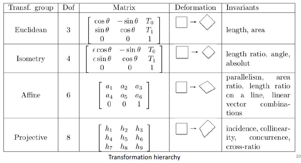
• projective geometry
  • perspective deformation can be modeled with 2D projective transformation
  • Euclidean geometry $\subset$ affine geometry $\subset$ projective geometry
  • infinity is modeled in projective geometry – so even parallel lines intersect (in infinity)
  • ray (point) – set $\mathcal R_v$ of all vectors $kv$ with direction $v$
    • where $v\in\mathbb R^{n+1}\setminus\set{o},\ k\in\mathbb R^*$
  • projective space
    • vectors in $\mathbb R^{n+1}$ → projective space $\mathcal P^n$
    • two vectors $X,Y$ represent the same point if $X\sim Y$
    • we divide by the last coordinate
    • if the last coordinate is zero, the rays don't intersect the plane (the points are in infinity)
    • another intuition – using a sphere/dome
  • projective geometry – infinity
    • $(x,y,1)$
      • we move in direction $(a,b)$
    • $(x+\lambda a,y+\lambda b,1)\sim (\frac x\lambda+a,\frac y\lambda +b,\frac 1\lambda)$
      • for $\lambda\to\infty$, we get $(a,b,0)$
    • all lines with the direction $(a,b)$ meet in infinity – at point $(a,b,0)$
  • projective transformations
    • preserve incidence relationships – collinearity and concurence
      • concurrence … if two lines intersect at $p$, they will intersect at $Mp$ after applying the transformation defined by $M$
  • projective basis
    • set of $(n+2)$ points of $\mathcal P^n$, no $(n+1)$ of which are linearly dependent
    • example – canonical basis of $\mathbb R^{n+1}$, plus $(1,1,\dots,1)^T$
  • change of basis is a projective transformation
    • projection matrix $M$ is determined up to a scale factor
  • hyperplanes – $m$ linearly independent points form a projective space of dimension $m-1$
  • duality
    • two lines define a point, two points define a line
    • also in some other cases
  • exercises
    • find intersection $X$ of lines $L_1,L_2$
      • both lines must contain $X$ → $L_1X=0$ and $L_2X=0$
      • use cross product $X=L_1×L_2$
    • find line $L$ going through $X_1,X_2$ → similar reasoning (cross product)
  • conics – projective transformations of the circle (“infinity line” touching the parabola and intersecting the hyperbola)
  • transformation groups
    • Euclidean (allows shift and rotation)
    • isometry (allows resizing)
    • affine
    • projective – only 8 DOF, because it is invariant to scaling
  • exercises
    • homography defined by 4 point correspondances
      • homography … projective transformation matrix
      • to move from 3 variables “up to scale” to 2 variables, we divide by the third variable (if its nonzero) and assume it's 1
        • we need to consider that it could be zero → similarly, we then divide by the second variable (so the second variable is 1 and the third variable is 0)
        • so we need to consider several situations
          • $p_z'\neq 0$
          • $p_z'=0$
          • only $p'_x\neq 0$
      • then we just write $P'\sim HP$ which corresponds to $\gamma(u,v,1)^T=H\cdot (x,y,1)^T$
        • $\gamma u=h_1x+h_2y+h_3$
        • $\gamma v=h_4x+h_5y+h_6$
        • $\gamma=h_7x+h_8y+h_9$
      • this can be rewritten as
        • $u(h_7x+h_8y+h_9)=h_1x+h_2y+h_3$
        • $v(h_7x+h_8y+h_9)=h_4x+h_5y+h_6$
      • and rearranged as two linear equations with 9 variables “up to scale” (so 8 variables)
      • so we need 4 correspondances to get 8 equations
      • refer to CMU slides for the entire procedure
    • for a homography $H$ transforming points, the associated transformation for lines is $H^{-T}$
      • $\ell^Tx=0$
      • $\ell^TH^{-1}Hx=0$
      • $(H^{-T}\ell)^THx=0$
    • affine transformation preserve parallelism
      • parallel lines … $L_1\times L_2=(x,y,0)^T$
      • $L_1'\times L_2'=H(x,y,0)^T$
      • if $H$ is affine transformation, it preserves the last 0 (projective transformation might not preserve it)
• 3D geometry
  • elementary transformations
    • translation $T=\begin{bmatrix}1&0&0&T_x\\0&1&0&T_y\\0&0&1&T_z\\0&0&0&1\end{bmatrix}$
    • rotations $R=R_z\cdot R_y\cdot R_x$
      • $\det R=1$
      • $R^{-1}=R^T$
      • $R_{x}=\begin{bmatrix}1&0&0&0\\0&\cos\theta &-\sin\theta &0\\0&\sin\theta &\cos\theta&0\\0&0&0&1\end{bmatrix}$
      • $R_{y}=\begin{bmatrix}\cos\theta &0&\sin\theta &0\\0&1&0&0\\-\sin\theta &0&\cos\theta&0\\0&0&0&1\end{bmatrix}$
      • $R_{z}=\begin{bmatrix}\cos\theta &-\sin\theta &0&0\\\sin\theta &\cos\theta&0&0\\0&0&1&0\\0&0&0&1\end{bmatrix}$
  • perspective projections
    • into the optical centre
    • focal length $f$ … distance between the projection centre and the image plane
    • image point $(x,y,z{=}f)$, world point $(X,Y,Z)$, optical axis $z$
      • here, we consider that the origin of the axes and the projection centre are the same point
    • perspective projection matrix $\begin{bmatrix}1&0&0&0\\0&1&0&0\\0&0&1&0\\0&0&1/f&0\end{bmatrix}$ to get an image point from a world point
      • can be deduced using intercept theorem (triangle similarity)
      • so $x=fX/Z$ (and $y=fY/Z$)
    • parallel lines intersect at infinity – this location defines a vanishing point in the image
      • for lines in a plane, vanishing points define a horizon line
  • parallel projections (ortographic)
    • projection is perpendicular to the image plane
    • we simply remove one coordinate (set to zero)
    • as if $f\to+\infty$
  • exercise
    • you have a projection matrix $P$
    • you move the camera or rotate it (you apply $T$), how does the new projection matrix look like?
    • $P'=TPT^{-1}$
      • first, we return to the original projection space using $T^{-1}$ (we move the point there)
      • we apply the projection $P$
      • then, we come back using $T$
      • sanity check: consider a zero transformation (e.g. for a parameterized rotation matrix, set $\alpha=0$) → it should hold that $P\sim P'$
      • note: the (projected) size of the object is proportional to its distance from the optical plane
        • so if we turn the camera (while keeping the focal length), the object gets smaller or larger
        • vertigo effect: you move the camera (toward or away from an object) and update the focal length to make the object appear the same size (but the background changes)
• camera models
  • most used camera model – pinhole model (perspective projection)
  • full transformation composed of
    • rigid transformation: world coordinates → camera coordinates
      • both 3D, only rotation & translation
    • perspective projection into the retinal plane (2D)
      • see matrix above
    • 2D transformation: retinal coordinates → image pixel coordinates
      • shift & scale
  • these transformations can be written as matrix multiplication
    • leftmost is the last one (retinal → image)
    • the third row is useless – we can remove it
    • also the perspective projection can be removed
    • so we get global transformation matrix $M\sim(K\cdot R\quad K\cdot T)$
      • $K$ … 3×3 intrinsic parameter matrix (shift & scale)
      • $R,T$ … 3×4 extrinsic parameter matrix (camera location)
    • a camera can be therefore described by 11 parameters (3×4 projective matrix)
    • we need 5.5 correspondences (3D to 2D) to estimate $M$

Applied 3D Vision

• panoramic mosaics
  • we assume all the images are taken from the same viewpoint
  • we apply homography
    • we need four correspondances to estimate it
    • we can use least squares if we have more than four
  • we can remap all the images onto one image plane by combining transformations (so we don't need correspondances for every pair of planes)
  • photometric mapping needs to be applied to make colors consistent
  • there may be some artifacts as a result of geometric errors
• two view geometry
  • in theory: if we have 2 image projections of the same 3D point, we can estimate its position by triangulation
  • in practice: the two rays usually don't cross (due to the noise)
    • algebraic approach: use least squares to solve an overdetermined system of equations
    • geometric approach: find the closest point to the 2 viewing lines
      • $(X,Y,Z)^T=C_i+\lambda_iD_i+\frac d2D_j×D_i$
      • $(X,Y,Z)^T=C_j+\lambda_jD_j-\frac d2D_j×D_i$
      • so $C_i-C_j+\lambda_i D_i-\lambda_jD_j+d(D_j\times D_i)=0$
        • $C_i,C_j$ … cameras (image centers)
        • $D_i,D_j$ … directions of the rays
        • $d$ … distance between the rays
        • 3 unknowns $\lambda_i,\lambda_j,d$
  • epipolar geometry
    • a point in the first image has to be on a certain line in the second image
    • this epipolar constraint is symmetric
    • epipolar line (seen by the second camera) is the projection of the viewing ray (of the first camera)
      • so all the epipolar lines go through a point (the epipole) – the projection of the other image center (= first camera)
      • we can also estimate the projection of the point in infinity
    • using these two points (epipole and “infinity”), we get the epipolar line $L\sim F_{ji}p_i$
      • $p_i$ … a point in the first image
      • $F_{ji}$ … fundamental matrix
    • the epipolar constraint between two corresponding points is then $p_j^T\underbrace{F_{ji}p_i}_L=0$
      • $F^T_{ji}=F_{ij}$ … fundamental matrix defining epipolar lines in image $i$ for points in image $j$
    • fundamental matrix … 3×3 matrix
      • captures all the geometric information between two images
      • is singular
        • maps points to lines (is one-to-many)
        • has a kernel $F_{ij}e_j=0$
        • in practice has rank 2
      • every correspondence gives us only one equation (equal to 0)
      • so we need 8 correspondences
      • but without any additional constraint, the estimated matrix will not be singular
    • essential matrix – takes calibration $K_i,K_j$ into account
      • $E_{ji}\sim K_jF_{ji}K_i$
• robust estimation
  • RANSAC … random sample consensus
  • we randomly select a set of observations, fit our model, and count outliers (points with distance $\gt$ threshold)
    • we run $n$ iterations and keep the best model (with the least outliers)
  • probability estimation
    • $w$ … proportion of good data
    • $n$ … sample size
    • $k$ … number of draws
    • $w^n$ … probability to get $n$ good points
    • $(1-w^n)^k$ … probability that $k$ draws are not good
    • we want the probability to get a good sample to be higher than $p$
      • $1-p=(1-w^n)^k$
      • $k\gt \ln(1-p)/\ln(1-w^n)$

Shape Modeling

• motion capture systems using markers
  • markers provide sparse motion information
  • no information on complete shapes or their appearances
• relief perception – two nearby viewpoints
  • hologram – relief image
• 3D video can be observed from any viewpoint (so 3D cinema is not really 3D)
• 4D modeling issues
  • acquisition issues – cameras with different modalities
  • shapes and appearances – need to be learned over time
  • recovering robust motion information, modeling and analyzing motions/gaits
• multi-view platforms
  • input: multi-view videos
  • output: 4D representations
• shape representation models
  • point clouds
    • usually correspond to the output of sensing devices
    • we don't know what is inside/outside, we don't have surfaces (but there are algorithms we can use to get surfaces)
  • voxels
    • 3D occupancy grid
    • complexity proportional to the size of the box
    • we usually want to first find the shape and modify the size of the box accordingly
    • we can use marching cubes to get a surface model (mesh)
  • 3D meshes
    • similar to point cloud but we have connectivity (often triangles)
    • we can easily attach textures
    • discretization attached to the shape (so simpler shapes can be discretized only using a few triangles)
    • Irregular Data Grid – mesh is a graph with nodes (vertices), edges (between neighboring vertices), and faces (often triangles)
  • image based
    • no explicit 3D model
    • we generate new image based on existing images
    • the set of images has to be calibrated (position and orientation data need to be stored), so that we can properly generate the new ones
    • appearance implicitly handled by the model
    • discretization attached to images
    • parallax occlusions difficult to handle without going to 3D
  • implicit
    • the object is described by a function $f:\mathbb R^3\to\mathbb R$
    • points with a constant value define surfaces (level-sets)
    • explicit meshes can be extracted (using marching cubes algorithm)
    • no explicit correspondences between different shapes
    • used in ML (functions can be learned by MLPs)
• traditional generative 3D-4D modeling pipeline (without prior model)
  • image acquisition → primitive extraction & calibration → shape construction → shape tracking → 3D-4D model
  • appearance of the model is based on the initial image and the constructed shape
• silhouette
  • extraction
    • chroma keying (blue or green background)
      • problem: white clothes, sweat, … tend to reflect green
    • background subtraction (static background)
      • take a photo without the object, take a photo with an object → what has changed?
      • problems: color ambiguities between background and foreground objects, luminosity changes, …
    • we can also use U-Net
  • from silhouettes to shapes
    • visual hull
      • the observed object is contained
      • some points are touching
    • voxel carving algorithm
      • we start with each voxel full (equal to 1)
      • we project every voxel into every camera (using the corresponding projection matrix)
        • we set it to zero if the pixel is outside of the silhouette for the given camera
        • note: usually, the cameras are not orthographic, they have an optical centre
      • notes
        • camera images have origin in the top left corner
        • pixel with coordinates $(32,10)$ … column 32, row 10
          • in a matrix, it's vice versa
    • convex shapes are difficult to carve
      • we can put camera inside the shape – but it is impractical (wiring, safety, etc.), also not general
• getting 3D points
  • active system: depth camera
    • we can use a structured light projector (projects “stripes” so that we can detect depth), calibration model is the same as for a camera
    • time of flight cameras – measure light travel from source to 3D scene and back
    • stereovision cameras – 3D point matched in 2 images
  • passive system: multi view stereo (with color)
    • more than 2 cameras
    • we construct depth map using photoconsistency
    • challenge: occlusion (there is some other object visible from a different angle – it's blocking the view of a certain camera)
  • some platforms are using both systems
  • active systems have inherently more limitations than passive ones

Deep Learning

• non-linear transformations applied to the input data
• we compose simple functions and create complex functions
• CNNs
  • convolutions with learned kernels
  • pooling to enforce invariances
    • we want translation equivariance (detect the object wherever it is on the image)
  • one layer usually consists of 1) convolution, 2) non-linearity, 3) spatial pooling, 4) normalization
• AlexNet
  • 8 layers in total
    • convolution & pooling – layers 1, 2, 5
    • convolution only – 3, 4
    • fully connected – 6, 7
    • output layer (with softmax) – 8
  • learned on ImageNet (1000 categories, 1.2M training images, 150k test images)
• The Bitter Lesson (essay) – instead of trying to build our domain knowledge into AI, we should build better models so they can learn it themselves
• training: gradient descent, backpropagation, parallelism on GPU
• encoder/decoder (autoencoder) architecture – useful for segmentation, getting 3D based on 2D
• McCulloch-Pitts neuron – $n$ binary inputs, one binary output (result of $\sum_i x_i\geq\theta$ for a threshold $\theta$)
• Frank Rosenblatt Perceptron
  • $wx+b\gt 0$
  • update: $w_i\leftarrow w_i+\alpha(t_j-y(x_j))x_{j,i}$
  • problem: non linear separable set (algorithm does not terminate), e.g. XOR
    • MLP solves that
• activation functions: linear, logistic (sigmoid), tanh, ReLU, GELU
  • without non-linearity, the network could be written only using 2 layers (without hidden layers)
  • continuous function can be approximated with a linear combination of translated/scaled ReLU functions
• gradient descent
  • $w\leftarrow w-\alpha\nabla E(w)$
  • SGD – only use subset to compute loss
  • backpropagation – previous computations can be reused (are needed because of chain rule)
• initialization of weights using small random values
• families of NNs: MLP, CNNs, autoencoders & VAEs, generative adversarial networks (GANs), RNNs & long short temporal memory (LSTMs), graph neural networks (GNNs), transformers
• bias–variance tradeoff (undefitting × overfitting)
• methodology – in general
  • state the problem you want to solve
    • classification, regression, segmentation
    • state input and output
    • narrow down the application domain
  • choose a “vanilla” architecture
  • choose the losses
  • evaluate properly (cross validation, train/validation sets)
  • be aware of (and explore) the biases in the datasets
  • push the boundaries

Deep Learning Architectures

• CNNs, pooling, normalization
  • 32×32×3 image & 5×5×3 filter → 28×28×1 output
  • striding, padding, dilation (spaces between convoluted pixels)
  • max and average pooling are most common
  • normalization – idea: output of the linear combinations must follow a standard Gaussian distribution (zero mean, unit variance)
• CNN architectures
  • LeNet – images of size 32×32
  • AlexNet – 224×224
  • VGG – only small 3×3 filters, more layers than AlexNet
  • GoogleNet Inception
    • very deep
    • problem: gradient vanishing
    • solution: intermediate losses are used
  • ResNet
    • solution: skip connections
  • U-Net
    • convolution/deconvolution architecture for segmentation
    • skip connections from intermediate representations to deconvolutions (across the U shape)
• object detection
  • two-stage detection: 1) is there something? (where?) 2) what is it?
    • R-CNN (region CNN) – extract regions, classify
      • problems: too many regions (slow), extracting regions is not learning-based
    • Fast R-CNN – first compute convolutions for the entire image, then look at regions (convolutions don't have to be computed separately for each region)
    • Faster R-CNN – learns to predict the regions of interest
    • Mask R-CNN – predicts a binary mask for each detected object
  • one-stage detection
    • Yolo (you only look once)
    • class probabilities, bounding box prediction (with confidence)
    • v4 uses mosaic augmentation (combining several annotated images into a mosaic and using it for training, makes the model more robust)
• generative models
  • autoencoder
    • learns a representation (encodings) of unlabeled data
    • dimensionality reduction (ignoring insignificant data)
    • usual technique for dimensionality reduction: PCA
      • limitation: we cannot do non-linear reparametrization (like switching from Cartesian to polar coordinates)
    • encoder → code (“bottleneck”) → decoder
    • code size is very important
      • too big → overfit, lack of interest
      • too small → loss of information
    • denoising AE
      • add noise to input image
      • pass through network
      • measure reconstruction loss against original image
    • for PCA, we can interpolate (we can safely take a point between too points and it's meaningful)
    • generally, AEs can lead to an irregular latent space (with no meaningful interpolation → close points in the latent space are not similar when decoded)
    • we want to regularize the latent space to enable generation → variational AE
      • so an input is encoded as a distribution (not as a point) in the latent space
      • regularization using KL-divergence
        • closed form for two normal distributions
      • the decoder then decodes a sample from the distribution
      • the loss consists of the distance of the decoded image from the original and the KL divergence of the encoded distribution from the $N(0, I)$ distribution
      • how to sample to allow backpropagation?
        • reparametrization trick
        • instead of sampling $z$ from $N(\mu_x,\sigma_x)$, we always sample $\zeta$ from $N(0,I)$ and then compute $z=\sigma_x\zeta+\mu_x$
          • so we can differentiate $z$ (and backpropagate)
      • limitation: images are blurry
  • generative adversarial network
    • generator, training set, discriminator
    • trying to match the real distribution
    • goal: fool the discriminator
  • GANs get sharper images than VAEs
    • VAEs use mean square error, producing sharp edges is not worth the risk
    • GAN discriminator can easily spot blurry images
  • diffusion models
    • slowly destroy structure in data distribution by adding noise
    • parameter $\beta_t$ (for time $t$) that governs the noise distribution (Gaussian)
      • its schedule affects the learning
    • the model tries to remove the noise
      • only step by step to improve stability
    • trained using U-Net (with adjustments)
    • can be conditioned with other inputs (other images, text, style, …)
      • then $\epsilon$ gets another parameter
      • Stable Diffusion uses CLIP to transform text into embeddings for conditioning
    • ways to make diffusion faster – distillation, one step diffusion
  • diffusion vs. GANs
    • training stability
      • GAN's optimum is a saddle point (min max)
      • diffusion is more stable
    • diversity
      • GANs have a risk of mode collapse (generating just one type of output)
      • diffusion models the distribution
    • cost & memory
      • GANs – fast, medium memory
      • diffusion – slow, high memory
    • conditional generation – diffusion outperforms GANs
• recurrent neural networks
  • for sequences, persistence
  • problem of long-term dependencies
  • long short-term memory
    • we are updating the state with multiplication and addition
    • forget gate: is this worth remembering (multiplying by a number $\in[0,1]$)
    • input gate: what new information are we storing in the cell state
    • output gate: output of the cell
  • variants: peephole connections (let gate layers look at the cell state), grouping forget and keep gates, GRU (gated recurrent unit)
  • types: one to one, one to many, many to one, many to many (2×)
  • problems
    • GRU still forgets stuff (especially with long sequences)
    • processing is sequential, hard to parallelize on GPUs
  • → Transformer architecture
• existing tasks are solved (to some extent)
  • new tasks need to be created → ARC-AGI datasets

Paper Session 2

• ViT
  • self-attention can be as expressive as convolutional layer
  • image split into patches
  • encoder-only Transformer, learned position embeddings (capture relative distances of patches)
  • needs enough data to learn patterns (in CNNs, there is inductive bias)
• DINO
  • emerging properties in self-supervised vision transformers
  • ViT limitations
    • supervised labels are coarse (one image – one label)
    • no explicit pressure to learn object boundaries, parts vs. background, spatial grouping
  • idea: use self-supervised pre-training
    • knowledge distillation with no labels
  • different crops
    • teacher gets only global
    • student gets all crops
    • → enforce local-to-global correspondences
  • to avoid mode collapse – centering and sharpening applied to the teacher's output
    • we are forcing the teacher to “be creative” when predicting distribution
    • sharpening prevents the distribution from being flat
    • centering prevents the distribution to always peak at the same place (by computing a running average)
  • setup
    • MLP on top of [class] encoding (like in ViT) → distribution
    • goal: minimize cross-entropy between student and teacher
• hi-res stereo datasets with subpixel ground truth (Middlebury)
  • capturing objects with stereo camera
  • how to create such datasets
  • two rounds of calibration (using checkerboard)
  • code images to get depth
  • ambient images
  • imperfection – useful for evaluation (real-world images are not perfect)
    • nothing in the world is perfect
• pose reconstruction
  • SMPL body model – shape & pose
  • two approaches
    • regression – predicts shape & pose based on the image
    • optimization – optimizes shape & pose based on camera parameters and ground truth of 2D joints (and initial shape & pose)
  • SPIN combines both
    • initializes optimization with regression outputs
    • uses optimization to supervise regression

Practical Units

Augmented Reality

• detection – detecting, refining, and drawing the projected image points of the checkerboard from a captured image
  1. implement simple checkerboard spot detection with findChessboardCorners on grayscale version of the input image
  2. draw the checkerboard points on the color input image with drawChessboardCorners.
  3. the points from question 1 can be improved in precision by refining based on a local window around the initial detections (before drawing the checkerboard points, add the refinement step using cornerSubPix)
• calibration, positioning
  1. calibrate the camera using calibrateCamera (3D to 2D matches at every detection that will be given to this function)
  2. find the camera extrinsics using solvePnPRansac
  3. use projectPoints to find the 2D reprojections of the 3D points using the estimated intrinsics and extrinsics to check that the result is correct
• drawing using reprojected points
  • the coordinates of a 3D cube are provided which you can use as initial augmentation object, but you can draw whatever you wish (use circle, line, drawContours for this purpose)

3D Shape Modeling

• at the beginning of the file the calibration matrices for the $12$ silhouette cameras are stored in the array $calib$ – each matrix corresponds to a $3\times 4$ linear transformation from 3D to 2D
• then the voxel 3D coordinate arrays $X, Y, Z$ and the associated occupancy grid, that shall be filled with $0$ or $1$, are defined
• grid resolution can be modified with the parameter resolution (if you program is too slow, you can reduce the resolution)
• training MLP to capture implicit representation
  • input: $x,y,z$
  • output: occupancy (0 or 1)
  • training based on the voxel representation

Segmentation – HourGlass vs. U-Net

• HourGlass – autoencoder with convolutions and deconvolutions, has bottleneck
• U-Net was invented to address precision problems of the original hourglass network
  • provides skip connections from intermediate representations